Essential Computational Thinking
Essential Computational Thinking: Computer Science from Scratch follows a CS0 breadth-first approach that is most appropriate for highly-motivated undergraduates, non-CS graduate students, or non-CS professionals.
Essential Computational Thinking
Computer Science from Scratch
by Ricky J. Sethi © 2020
ISBN-13: 978-1516583218
ResearchGate
(PDF)
Published and distributed by Cognella Academic Publishing
and also available on Google Books and Amazon.
Index
- PowerPoints
Table of Contents with PowerPoints and recorded lectures for Ch. 3 - 7
- Companion Video Series
A video series consisting of 8 episodes that complements Ch. 0 - 2
- Auto-Graded Programming Problems
A set of auto-graded Python programming exercises that complements Ch. 3 - 7
- Preface
Preface from the text including target audience
- Excerpts
Some relevant excerpts from the text, including Computational Thinking Overview and Definition
- Key Images
Some key images from the text
- Errata
Updated list of errata for the text
PowerPoints
PowerPoints and Recorded Lectures
Table of Contents with PowerPoint slides and Recorded Lectures for various chapters.
Part I: Theory: What is Computer Science?
-
- What is Knowledge?
- Declarative vs Imperative Knowledge
- The Key to Science
- Computer Science: The Study of Computation
- A Review of Functions
- Computable Functions
- Talking in Tongues: Programming Languages
-
Computational Thinking and Information Theory
- What is Thinking?
- Deductive vs Inductive Thinking
- Thinking About Probabilities
- Logical Thinking
- Computational Thinking and Computational Solutions
- Two Fundamental Models of Programming
- Pseudocode
- Functional and Imperative Models of Computation
- Information Theory
- Shannon's Information Entropy
-
Computational Problem Solving
- What is a Model?
- Data Representations
- Number Representations
- Digital Representations
- Boolean Algebra
- What is Information Processing?
- What is Computer Information Systems (CIS)?
- Programming Languages
- Computational Thinking
- Problem Space and System State
- Computational Thinking in Action [PPTX]
-
Computational Thinking and Structured Programming [PPTX]
- Review of Computation
- Computational Thinking Basics
- Minimal Instruction Set
- Getting Started with Python
- Syntax, Semantic, or Logic Errors
- State of a Computational System
- Natural vs Formal Languages
- Translating your programs
- Playing with Python
- An example using Computational Thinking
-
- Different Types of Data
- Data Type = Values + Operations
- Variables and Expressions
- Input/Output
- An Example Using Computational Thinking
-
- Algorithms and Control Structures
- Sequence
- Selection
- Repetition
- An Example Using Computational Thinking
-
- Abstract Data Types
- A Non-Technical Abstract Type
- Advantages of ADTs
- Data Structures
- Strings
- Lists and Tuples
- An Example Using Computational Thinking
-
- Functions Redux
- Functions in Python
- Sub-routines with parameters and values
- Namespaces and Variable Scope
- Exception Handling
- File I/O
- An Example Using Computational Thinking
-
- Zen and the Art of Object-Oriented Programming
- The Road to OOP
- Solving Problems with Software Objects
- What is Java?
- Data Structures and I/O in Java
-
Databases and MDM
- Mind Your Data
- Database Management
- Relational Database Model
- Database Modeling and Querying
- Normalization
-
Machine Learning and Data Science
- Computational Thinking and Artificial Intelligence
- Getting Started with Machine Learning
- Elements of Machine Learning
- Data Science and Data Analytics
- Bayesian Inference and Hypothesis Testing
- The Entropy Strikes Back
- Learning in Decision Trees
- Machine Learning, Data Science, and Computational Thinking
-
Computational Complexity
- Big O Notation
- Searching and Sorting Algorithms
- P vs NP
- Ch. 0: On The Road to Computation
- Ch. 1: Computational Thinking and Information Theory
- Ch. 2: Computational Problem Solving
- Ch. 3: Computational Thinking and Structured Programming
- Lesson 1: Input, print and numbers
- Ch. 4: Data Types and Variables
- Lesson 2: Integer and float numbers
- Ch. 5: Control Structures
- Lesson 3: Conditions: if, then, else
- Lesson 4: For loop with range
- Lesson 6: While loop
- Ch. 6: Data Structures
- Lesson 5: Strings
- Lesson 7: Lists
- Lesson 9: Two-dimensional lists (arrays)
- Lesson 10: Sets
- Lesson 11: Dictionaries
- Ch. 7: Procedural Programming
- Lesson 8: Functions and recursion
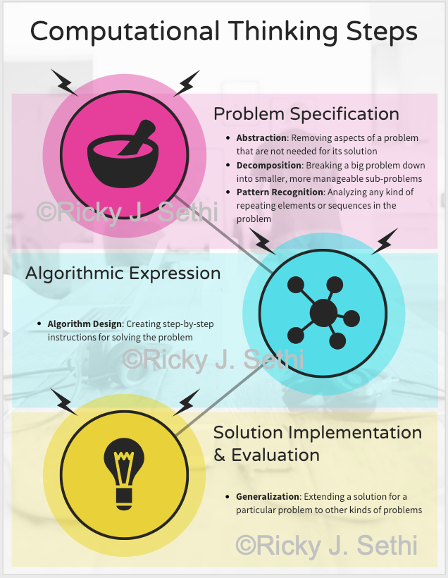
- Problem Specification: We'll start by analyzing the problem, stating it precisely, and establishing the criteria for solution. A computational thinking approach to solution often starts by breaking complex problems down into more familiar or manageable sub-problems, sometimes called problem decomposition, frequently using deductive or probabilisic reasoning. This can also involve the ideas of abstraction and pattern recognition, both of which we saw in our temperature sensor problem when we found a new representation for our data and then plotted it to find a pattern. More formally, we'd use these techniques in creating models and simulations, as we'll learn later on.
- Algorithmic Expression: We then need to find an algorithm, a precise sequence of steps, that solves the problem using appropriate data representations. This process uses inductive thinking and is needed for transferring a particular problem to a larger class of similar problems. This step is also sometimes called algorithmic thinking. We'll be talking about imperative, like procedural or modular, and declarative, like functional, approaches to algorithmic solutions.
- Solution Implementation & Evaluation: Finally, we create the actual solution and systematically evaluate it to determine its correctness and efficiency. This step also involves seeing if the solution can be generalized via automation or extension to other kinds of problems.
-
The scientific method is usually written out as something like: ↩︎
- Observe some aspect of the universe
- Use those observations to inform some hypothesis about it
- Make some prediction using that hypothesis
- Test the prediction via experimentation and modify the hypothesis accordingly
- Repeat steps 3 and 4 until the hypothesis no longer needs modification
- Problem Specification: analyze the problem and state it precisely, using abstraction, decomposition, and pattern recognition as well as establishing the criteria for solution
- Algorithmic Expression: find a computational solution using appropriate data representations and algorithm design
- Solution Implementation & Evaluation: implement the solution and conduct systematic testing
- Problem Specification
- Computational Thinking Principles: Model Development with Abstraction, Decomposition, and Pattern Recognition
- Computer Science Ideas: Problem Analysis and Specification
- Software Engineering Techniques: Problem Requirements Document, Problem Specifications Document, UML diagrams, etc.
- Algorithmic Expression
- Computational Thinking Principles: Computational Problem Solving using Data Representation and Algorithmic Design
- Computer Science Ideas: Data representation via some symbolic system and algorithmic development to systematically process information using modularity, flow control (including sequential, selection, and iteration), recursion, encapsulation, and parallel computing
- Software Engineering Techniques: Flowcharts, Pseudocode, Data Flow Diagrams, State Diagrams, Class-responsibility-collaboration (CRC) cards for Class Diagrams, Use Cases for Sequence Diagrams, etc.
- Solution Implementation & Evaluation
- Computational Thinking Principles: Systematic Testing and Generalization
- Computer Science Ideas: Algorithm implementation with analysis of efficiency and performance constraints, debugging, testing for error detection, evaluation metrics to measure correctness of solution, and extending the computational solution to other kinds of problems
- Software Engineering Techniques: Implementation in a Programming Language, Code Reviews, Refactoring, Test Suites using a tool like JUnit for Unit and System Testing, Quality Assurance (QA), etc.
- Data: structure raw facts for evidence-based reasoning
- Representation: create a problem abstraction that captures the relevant aspects of the system
- Algorithm: delineate a systematic procedure that solves the problem in a finite amount of time
Disclaimer: correlation does not equal causation; even if you spot a pattern, you might want to confirm or validate that prediction with other analyses before actually putting your money where your pattern is.↩︎
- Computer Science emphasizes theoretical and empirical approaches to manipulating data via computation or algorithmic processes.
- Informatics deals with a broader study of data and its manipulation in information processes and systems, including social and cognitive models.
- Data Science tackles structured and unstructured data and uses both computational methods and cognitive or social methods, especially when visualizing complicated data analytics.
- Analyze historical trends
- Forecast future outcomes
- Assist decision making with actual quantitative predictions
- Exploratory Data Analysis (EDA) mainly asks, "What happened in the past?" It thus analyzes historical data and, in the BI/BA paradigm, is called Descriptive Analytics.
Descriptive analytics tells us what happened; this involves using data to understand past and current performance to make informed decisions. This is sometimes said to include Planning Analytics, where the plan for the forecasted goals is established, including planning and budgeting concerns. - Data Analysis tries to answer, "What could happen in the future?" In the BI/BA paradigm, this is called Predictive Analytics and, sometimes, also called Business Informatics when it addresses organizational behaviour/science and systems, as well. Usually, this involves building a machine learning model to predict an outcome.
Since predictive analytics deals with what could happen, it will involve using historical data to predict future outcomes. This sometimes also includes Diagnostic Analytics, which looks at why things happened in the past using data mining and data discovery to also establish correlations, causal relationships, and patterns in historical data. The focus is mainly on processing existing data sets and performing statistical analyses on them.- Data analysis involves using machine learning algorithms to derive insights and support decision-making. This also requires extracting, cleaning, and munging data in order to transform it into a useable format for modeling that data to support decision-making and confirming or informing conclusions. Cleaning and munging the data involves dealing with missing fields and improper values, as well as converting raw files to the correct format and structure.
- Data Science answers the question, "What should we do next?" It uses predictions and helps decide what to do next and how to make it happen. In the BI/BA paradigm, it is called Prescriptive Analytics.
In essence, prescriptive analytics looks at what you can do about what's about to happen; this involves a consideration of what we can do about what's going to happen and how we can make it happen; prescriptive analytics sometimes concentrates on optimization and tries to identify the solution that optimizes a certain objective.- Data science requires the user to be able to innovate algorithms, find unique, additional data sources, and have deep domain knowledge. It uses ideas from computational science and information systems in order to gain actionable insights and make predictions from both structured and un-structured data about what to do or which decisions to make. This is why a data scientist should also have some domain knowledge in addition to the ability to create machine learning models and identifying ways to predict trends and connections by exploring novel, perhaps disconnected, data sources.
- Use k-fold cross-validation on your initial training data
- Add more (clean) data
- Remove some features from the model
- Use early stopping after the point of diminishing returns
- Add regularization to force your model to be simpler
- Add Ensemble learning of Bagging by using a bunch of strong learners in parallel to smooth out their predictions
- Add Ensemble learning of Boosting by using a bunch of weak learners in sequence to learn from the mistakes of the previous learners
- Problem Specification, which involves Abstraction, Decomposition, and Pattern Recognition
- Algorithmic Expression, which involves Algorithm Design
- Solution Implementation & Evaluation, which involves testing and Generalization
- Information Theory is a mathematical theory of information processing by classical or quantum processes.
Information is a measure of the decrease of entropy, or uncertainty, from the source to the receiver. - Shannon's Information Function, \( h(p) = log_2(\frac{1}{p}) = -log_2(p) \), is a measure of the inverse of the probability which we can call the uncertainty, or surprise: the smaller the probability, the higher the uncertainty (and the higher the surprise if that event occurs).
-
Shannon's Information Entropy, \( H = -\sum_i^N p_i log_2(p_i) \), is a measure of the average uncertainty, or the average of the surprise, associated with all the possible observations. It is a measure of the average of the Shannon Information Function per observation, or symbol: the sum of the Shannon Information Function for each observation weighted by the probability of that observation. The higher the entropy, the higher the Shannon Information Function value of a system.
- Shannon used H for entropy as H is used for entropy in Boltzmann's H-theorem, a continuous version of Shannon's discrete measure.
-
Shannon Information is then a measure of the decrease in entropy, or decrease in uncertainty/surprise, at the receiver's end:
Information = Rate of Transmission = \( H_\text{before} - H_\text{after} \)
Here, Hbefore is the uncertainty before the observation, or before receiving the message, and Hafter is the reduction in uncertainty, which can only be 0 for noiseless systems. In one sense, Information can be thought of as a measure of the decrease in entropy between two events in spacetime.- The conditional entropy, Hy(x), which measures the average ambiguity of a signal on the receiver's end, is called equivocation by Shannon (p. 20 of Shannon's seminal paper). The conditional entropy is also called missing information by Shannon.
- A data model is a conceptual, abstract model that organizes how data is represented and how the data elements relate to each other
-
A data type is a logical, language-independent expression of a data model and the associated operations that are valid on those data values
-
An Abstract Data Type (ADT) is a logical, language-dependent model of the data type, the data and its operations, but without implementation details
- A class is the logical representation of an Abstract Data Type utilized in a particular OOP paradigm
-
An Abstract Data Type (ADT) is a logical, language-dependent model of the data type, the data and its operations, but without implementation details
-
A data structure is the physical implementation of the data type in a particular language
-
The physical implementation of an abstract data type is also called a data structure since it helps organize a value that consists of multiple parts
- An object is the actual physical implementation of a class in a specific OO language
-
The physical implementation of an abstract data type is also called a data structure since it helps organize a value that consists of multiple parts
- Association Examples: a Customer USES-A Key or a Student USES-A Instructor
- Aggregation Examples: a University HAS-A Professor or Car HAS-A Passenger
- Composition Examples: an Arm IS-A-PART-OF Person or a Human OWNS-A Heart
-
Original Formulation: Why did the chicken cross the road?
The original formulation is ambiguous and overly broad: it doesn't indicate which chickens were involved, where they were located, what the weather and other environmental conditions were, etc. -
First Revision: How many chickens crossed Main St. last night at 3am and under what conditions?
This first iteration is a little better and you can answer it directly by just gathering the data and doing an initial analysis: this is the EDA and questions like these can be answered by simple statistical analysis. -
Final Formulation: Which contextual and environmental factors likely caused 30% of the chickens to cross Main St. between 1am - 3am on a rainy night with depleted food stores from the desert to the cornfield?
The final version is more precise and makes quantitative predictions (the probability or likelihood) of which factors motivated chickens to cross: was lack of food the most important factor? Was the weather a factor? Would more have crossed in sunnier weather? Did the night-time make them more confident? These are only the factors, or variables, we've identified so far, especially through our EDA. - Business Problem
It helps to start by first stating the business problem.
E.g., What factors are related to employee churn? Can we predict future terminations? - Initial Problem Statement
Then, convert that business problem into an initial problem statement by making it precise and quantitative and something you can use with a machine learning model.
E.g., Is there a correlation between age, length of service, and business unit with the terminated status of an employee?
In general, the initial problem statement should be precise and quantitative and is often expressed as some independent variables, the predictors, having a presumed correlation with some dependent variable, the response variable or class label. - Research Question
Once you have a precise, quantifiable question, you will have to fine-tune it to match one or more of the 8 kinds of questions that machine learning usually answers. Once you decide which of those questions it fits, you'll formulate your final research question.
E.g., How likely is it that someone under 50, with more than 20 years service, working in the IT Department will be gone within a year?
This would be an example of a regression task where you predict a number, a probability, but you can also convert it to a classification task where you predict a category label, whether that person belongs in category A or category B. - Find if there are any unusual data points: is this weird? → Anomaly Detection
- Discover how this is organized or structured? → Clustering and Dimensionality Reduction
- Predict a number, like how much or how many? → Regression
- Predict if something is A or B? → Binary Classification
- Predict if this is A or B or C or ...? → Multi-Class Classification
- Find the best way to make your next move; what should you do next? → Reinforcement Learning
- Is the data super-complicated and hard to understand? → Deep Learning
- Is accuracy quality really important? → Ensemble Methods
- Start by imposing several constraints to simplify the problem
- Do extensive EDA and get baseline results as the first approximation
- Relax some constraints and repeat the process for the more complex problem
- Decision Trees are interpretable but overfit (use ensemble RF instead)
- Neural Networks : non-linear relationships and resistant to curse of dimensionality but black boxes that are slow and susceptible to missing data and outliers
- Deep Learning: No need to do feature engineering or feature extraction but have a lot of parameters and take a long time to train and need a lot more data
- Start by picking a learning algorithm that's appropriate for the task at hand
- Use the Training Dataset to learn the algorithm's parameter values
- Use the Validation Dataset to tune the algorithm's hyperparameters and architecture — the resulting algorithm is the tentative model
- Use the Testing Dataset to gauge the tentative model's performance and, if no changes are needed, this is the final model
- Now you can apply the final model to unseen data to make your final prediction for that task
- Do data cleaning and data wrangling/munging on both the original dataset and the new, unseen data, including things like removing noise, normalizing values, and handling missing data.
- Split the original dataset into training, validation, and testing datasets.
- Subsequently, carry out feature engineering and hyperparameter tuning, as appropriate. Train your selected models on the training set and tune their hyperparameters using the validation set.
- Evaluate the trained models using appropriate metrics and use techniques like cross-validation to ensure the models' performance is consistent across different data subsets.
- Create the final model and use that final model to make your final prediction.
- Exploratory: identifying patterns
- Uses statistics and visualizations for Exploratory Data Analysis (EDA) to describe and get historical insights into the dataset
- Predictive: making informed guesses
- Uses machine learning methods for optimization and prediction of new data points with accuracy and precision
- Inferential: quantifying our degree of certainty
- Uses statistical inference to find correlations between variables, test hypotheses, or draw inferences about the population parameters
- Are you making predictions? If so, you'll do either Data Science or Data Analysis; otherwise, you'll do EDA.
- Will you use those predictions to make actionable decisions? If so, you'll do Data Science; otherwise, you'll employ Data Analytics.
- Is there any uncertainty involved? If not, you can just use EDA techniques.
- Are you using lots of high-dimensional data? If so, you'll need to use machine learning; otherwise statistical inference alone could work.
- Questions to ask for doing EDA:
- What decisions are you trying to make? What insights are you looking for?
- What questions can be answered with the data?
- What is the primary comparison you're trying to make in each visualization?
- What do you want the reader to take away from each visualization?
- How would you explain the visualization to someone who can't see it?
- Develop a research question: delineate what to predict or estimate: a precise, quantitative prediction that can be validated
- Gather the data: find or sample relevant datasets
- Understand the data: Exploratory Data Analysis: visualize data, detect anomalies, identify patterns
- Make the predictions: develop a predictive model by building, fitting, and validating the appropriate algorithm
- Communicate the results and recommendations: summarize results, evaluate if they are reliable and make sense using evaluation metrics, interpret results and predictions, possibly via storytelling
- Additional ML Models, including baseline like Naive Bayes, SVM, kNN, k-Means, Neural Networks, Decision Trees, etc.
- Especially Ensemble methods like Random Forest, Gradient Boost, AdaBoost, etc.
- Feature Engineering, Feature Importance,and Feature Selection: combine features, see which features are most relevant, dummy variables, one-hot encoding, etc.
- Dimensionality Reduction and Regularization: PCA, SVD, LDA, etc.
- Additional Metrics: accuracy, confusion matrix, heat map, EER, OOB error, etc.
- Classification Metrics: Accuracy, AP, MAP, Brier, F1, LogLoss, Precision, Recall, Jaccard, ROC_AUC, etc.
- Regression Metrics: Explained Variance Score, Max Error, Mean Absolute Error, Mean Squared Error (MSE), Mean Squared Log Error, Median Absolute Error, R2, Mean Poisson Deviance, Mean Gamma Deviance, RMSE, etc.
- Clustering Metrics: Elbow Method, Silhouette coefficient, BIC score with a Gaussian Mixture Model, etc.
- AutoML for hyperparameter optimization and model selection: especially Automated Machine Learning libraries like auto-sklearn, tpot, mlbox, etc.
- Stacking feeds the same original data to several different algorithms and the output of each of those intermediate algorithms is passed to a final algorithm which makes the final decision.
- Bootstrap AGGregatING (Bagging) uses the same algorithm on several different subsets of the original data that are produced by bootstrapping, random sampling with replacement from the original data. The result of each component is then averaged in the end.
- Boosting uses several different data subsets in a linear, sequential way rather than in a parallel way as in Bagging. Similar to Bagging, though, each subsequent algorithm is fed a subset of the original data that is produced by random sampling with replacement from the original data but, different from Bagging, the mis-classified data in the previous step is weighted more heavily in a subsequent step. As a result, the different algorithms are trained sequentially with each subsequent algorithm concentrating on data points that were mis-classified by the previous algorithm.
- Data are the organized observations of nature;
- Information involves quantifying the probability of occurrence associated with that data (e.g., via a transformation like Shannon's Information Function);
- Knowledge is the reduction in uncertainty (e.g., via a transformation like Shannon Information*, the difference between Shannon Information Entropies)
- General
- Fundamental Science
- Information Theory
- Databases
- Machine Learning
- GENERAL
- Structured values in some representation
- FUNDAMENTAL SCIENCE
- Quantitative observations of Nature
- INFORMATION THEORY
- Organized sequence of symbols representing ideas
- DATABASES
- Raw facts converted into structured data
- MACHINE LEARNING
- Abstracting datasets with pattern recognition via Exploratory Data Analysis/Descriptive Analytics
- GENERAL
- Data transformed into a particular context to reach a conclusion
- FUNDAMENTAL SCIENCE
- Prediction from a model-based hypothesis
- INFORMATION THEORY
- Assess probability of occurrence of data to predict amount of surprise*
- DATABASES
- Contextualize data into the logical model to predict organization
- MACHINE LEARNING
- Algorithmic model’s predictions via Data Analysis/Predictive Analytics
- GENERAL
- Organized information for actionable, logic-based problem-solving
- FUNDAMENTAL SCIENCE
- Validating model’s predictions into a theory for wider applicability
- INFORMATION THEORY
- Calculate change in the entropy of a system to gauge information gain
- DATABASES
- Execute query on the physical model to help decide upon action
- MACHINE LEARNING
- Generalization for verifiable decisions via Data Science/Prescriptive Analytics
- * Shannon's Information Function, h(p)=-log2(p), would be a measure of the amount of surprise. Then, Shannon Information, the difference in entropies, Hbefore - Hafter, would be a measure of knowledge gained in this paradigm.↩︎
-
Page 282: add to beginning of Final Figure's Caption:
To summarize, then:
- Data are the organized observations of nature;
- Information involves quantifying the probability of occurrence associated with that data (e.g., via a transformation like Shannon's Information Function);
- Knowledge is the reduction in uncertainty (e.g., via a transformation like Shannon Information, the difference between Shannon Information Entropies)
-
Page 282: definition of variance should be different, as per below: it should say "given training dataset" not "given data point":
Variance error is how sensitive the model is to small fluctuations in the dataset. This is the error due to how much a target function's predicted value varies for a given training dataset.
Also, it should say, "Bias error measures how far off the predicted values are from the actual values and usually occurs when all the features are not taken into account." -
Page 282: after the bias variance equation, add:
Overfitting often occurs if your model does much better on the training dataset than the testing dataset. You can also check by using a very simple model as a benchmark to see if using more complex algorithms give you enough of a boost to justify their use. In general, to mitigate overfitting, you can:- Use k-fold cross-validation on your initial training data
- Add more (clean) data
- Remove some features from the model
- Use early stopping after the point of diminishing returns
- Add regularization to force your model to be simpler
- Add Ensemble learning of Bagging by using a bunch of strong learners in parallel to smooth out their predictions
- Add Ensemble learning of Boosting by using a bunch of weak learners in sequence to learn from the mistakes of the previous learners
-
Page 282: replace "so a lot of machine learning ends up tweaking" with "so a lot of supervised machine learning ends up tweaking".
-
Page 276: "The decrease in entropy is the same as a decrease in uncertainty (or an increase in the amount of surprise)" should be: "The decrease in entropy is the same as a decrease in uncertainty (or a decrease in the amount of surprise)"
-
Page 276: "We can generalize that decrease in uncertainty (or an increase in the amount of surprise) to a random variable itself: this lets us quantify the amount of information that we can potentially observe" should be: "We can generalize that decrease in uncertainty (or the decrease in the amount of surprise) to a random variable itself: this lets us quantify the amount of information that we can potentially observe"
-
Page 276: "Shannon Information, which is defined as \(h(x) = −log(p(x))\), reflects a decrease in uncertainty (or an increase in the amount of surprise) when that event x occurs: this is what we call the amount of information contained in a discrete event x that we can potentially observe." should be: "The Shannon Information Function, which is defined as \(h(x) = −log(p(x))\), reflects the amount of uncertainty (or the amount of surprise) associated with an event x: this is what we call the amount of potential information contained in a discrete event x that we can potentially observe."
-
Page 271: Supervised Learning: Regression: replace "MSAE," with "RMSE, MAE,"
-
Page 274: Add text box at bottom:
A Random Variable, \(X\), is a real-valued function that assigns a real number, \(x\), to each possible outcome in the sample space of an experiment or phenomenon. The Probability Distribution Function (PDF), \(Pr(X)\), also known as a Probability Distribution, assigns a probability to each possible outcome in the random variable's sample space. This \(Pr(X)\) comes in two flavours: either discrete (probability mass function) or continuous (probability density function). A probability mass function (pmf) describes the probability of a discrete random variable having a certain exact discrete value; a probability density function (pdf) describes the probability of a continuous random variable having a value that falls within a certain infinitesimal interval.
The Cumulative Distribution Function (CDF), \(F(x)\), also known as a Distribution Function, gives the probability that a random variable, \(X\), will take on a value, \(x\), within a certain range. The CDF of a discrete random variable can be calculated by summing its pmf while the CDF of a continuous random variable can be calculated by integrating its pdf, which results in a probability value, \(r\), for the random variable, \(X\), to have a value in the range bounded by \(x\): $$ r = F_{X}(x) = Pr(X \leq x) = \int_{-\infty}^x Pr(a)da $$ Sampling from a probability distribution means generating a sample/value, \(x\), from that probability distribution function, PDF. In order to sample from a distribution for some random variable \(X\), you need to be able to compute the CDF since sampling is done by first drawing a random sample, \(r\), from a Uniform Distribution on \([0,1]\) and then using the inverse CDF to transform that number, \(r\), into a sample, \(x\), from \(X\).
Since the CDF computes the area under the pdf, \(r\), for a certain value, \(x\), the inverse CDF calculates that value, \(x\), which is associated with a particular area under the pdf, \(r\). If you cannot calculate the CDF or inverse CDF, e.g., if the integral of the CDF is intractable, then you can instead use one of the many Monte Carlo Sampling methods to randomly sample a value, \(x\), from the probability distribution function, PDF.
We can sample/generate a value from a CDF programmatically for a discrete random variable, as well; you start by first generating a random number, \(r\), between 0 and 1 by using a Uniform Distribution. Then, you have to check the discrete CDF for various sample values, \(i\), until you find the one \(i\) for which \(F(i) \geq r\). The sample value \(i\) you find is then considered a random sample, \(x\), from that discrete pmf distribution, as in the following sample code:# For a discrete CDF, F import numpy as np def generate_sample_from_cdf(F): r = np.random.rand() for i in range(len(F)): if F[i] >= r: return i # Generate a sample value, x, from the synthetic discrete CDF, F, for pmf=(0.25, 0.25, 0.25, 0.25): F = np.array([0, 0.25, 0.5, 0.75, 1]) x = generate_sample_from_cdf(F)
The most general approach to sampling from a continuous probability distribution is to use transformation methods, with the most popular being a special case called the inverse transform method, or inversion. For a continuous random variable, the inversion method requires integrating the CDF. The general algorithm for generating a sample, \(x\), from a continuous CDF for a given pdf is:- Find the CDF, \(F(x)\)
- Get a random number from the uniform distribution \(r \sim U[0,1]\)
- Then, calculate the inverse CDF, \(F^{-1}(r)\), for the pdf associated with that random number, \(r\), to get a value, \(x\), drawn from that original CDF: \(x = F^{-1}(r) \sim F(x) \)
For an exponential pdf like \( \text{pdf}(x) = e^{-x} \), the CDF would be: $$ r = Pr(X \leq x) = F(x) = \int_0^x e^{-a} da = 1 - e^{-x} $$ Here, \(F(x)\) gives the area under the curve as \(r = 1 - e^{-x}\), for a certain value \(x\). The inverse CDF would then be \( F^{-1}(r) = - log(1 - r) = x \) and we can implement that in Python as follows:
# For an exponential CDF of a continuous random variable (which has the log() function as its inverse CDF)
import numpy as np
import matplotlib.pyplot as plt
def F_inverse(r):
  return( - np.log(1 - r) )

# Generate a sample value, x, 100 times from the inverse of the exponential CDF, F^-1:
#sampled_distribution = [F_inverse(np.random.rand()) for r in range(100)]
#sampled_distribution = [F_inverse(r) for i in range(100) if ((r := np.random.rand()))]
sampled_distribution = []
for i in range(100):
  r = np.random.rand()
  x = F_inverse(r)
  sampled_distribution.append(x)

# Plot that sampled distribution:
plt.hist(sampled_distribution)
plt.show()
Evaluating a probability distribution, on the other hand, generally involves delineating the properties of a distribution, things like its mean, variance, shape, etc., either by using analytical methods or by using Monte Carlo simulations, as we'll see in a bit. Sampling a distribution generates specific, individual values that can then be used as data for subsequent analyses whereas evaluating a distribution is often necessary to make predictions about that distribution itself. -
Page 269, Figure 10.21: Add further explanation:
Our Null Hypothesis was that they are NOT PREGNANT. So if the true state of nature is NOT PREGNANT (i.e., the Null Hypothesis is true), then, if we reject the null hypothesis based on the statistical analysis, that is a Type I Error (a False Positive). In our confusion table, we call the Null Hypothesis being true as the Actual underlying state of the system, which is NEGATIVE for the Actual Value in the column on the right.
Similarly, we call the Alternative Hypothesis being TRUE a POSITIVE when we are, in reality, PREGNANT (i.e., the Null Hypothesis is not true). In this case, if the statistical analysis concludes the Null Hypothesis is true, we have a Type II Error, where we have a FALSE NEGATIVE. -
Page 263: Add to footnote after "When you draw different samples from a population, the values of those variables will usually exhibit some random variation by virtue of picking different subsets of the underlying population."
There are two main approaches to sampling from a population: probability sampling and non-probability sampling. A sample drawn from the population consists of multiple observations or data points drawn from that population, the so-called sampling frame.
Probability sampling usually comes in four flavours:
- simple random sample: every data point in the population has an equal chance of being selected
- systematic sample: data points are chosen at regular intervals starting with a random starting point
- stratified sample: consists of dividing the population into sub-groups and then using random or systematic sampling to select a sample from each sub-group
- cluster sample: again dividing the population into sub-groups and then randomly selecting entire sub-groups
Non-probability sampling is easier to do but not every data point/observation has a chance of being included in these approaches. As such, there's a higher risk of sampling bias with these methods and the inferences about the population are weaker, thus making them more popular in exploratory or qualitative research applications. The main non-probability approaches are:
- convenience sampling: including only those observations that are most easily accessible
- voluntary response: where people either volunteer themselves or respond to surveys, thus introducing self-selection bias
- snowball sampling: where participants refer other participants
- quota sampling: where you divide the population into sub-groups and then set a limit, or quota, for the maximum number of observations that can be drawn from each sub-group
Once you have a sample from a population, you can compute descriptive statistics about that data. These measures, or statistics, like the mean, mode, etc., can be used as a rough estimate of the corresponding parameter of the underlying population. While descriptive statistics focuses on describing the characteristics of the sample from a population, inferential statistics draws conclusions about the underlying population based on the sample (drawn from that population). Inference usually comes in the form of confidence intervals, which give the probability of a parameter falling within a certain range, and hypothesis testing, which uses sample statistics to make inferences about the underlying population's parameters. It does so by using the sample statistics to calculate a test statistic in order to compare the differences between the parameters of two populations. This test statistic determines how likely it is that the difference between two sample statistics (like two sample means) is likely to differ from the true difference between the corresponding parameters of the underlying populations (e.g., the two population means).
The most common statistics used for a sample from a population, where a sample consists of multiple observations/data points drawn from that population, are the so-called measures of central tendency like mean, mode, and median. The median (the exact center of a distribution) and the mode (the most frequently occurring value in a distribution) are relatively straightforward while the mean is usually what we refer to as the average, where you add all the values and then divide by the number of observations.
In general, the mean balances the values in a distribution: i.e., if you subtract the mean from each value, and then sum the differences, it will result in 0. As such, you can think of the mean as that which minimizes variation of the values. Since the mean is the point around which variation of the values is minimized, if the differences between values and the mean are squared and added, then the resultant sum will be less than the sum of the squared differences between the values and any other point in the distribution. However the mean can be deceptive if the distribution has outliers.
You can compute such statistics on samples drawn from a population and, if you draw many such random samples from a population and then compile the statistic calculated for each sample, you will form a sampling distribution, which is also a probability distribution and has very interesting implications for the Central Limit Theorem, as we saw earlier.
-
Page 262: We can also think of the statistical power, \(\beta\), as the \( \text{Pr}(\text{True_Positive}) =(1 - \text{Pr}(\text{False_Negative})) \). Thus, a high statistical power means that we have a small risk of getting a \(\text{False_Negative}\) (Type II error); a low statistical power means we have a large risk of doing a Type II error. For example, if we use a normal distribution, then we can use the z-score values and calculate the sample size, \(n\), as:
$$ n = \left(\frac{Z_{1-\alpha/2} + Z_{1-\beta}}{|\mu_{H_a}-\mu_{H_o}|/\sigma}\right)^2 \Rightarrow \left(\sqrt{2} \sigma \frac{Z_{\alpha/2} + Z_{\beta}}{|\mu_{H_a}-\mu_{H_o}|}\right)^2 $$
Here, \(\alpha\) is the significance level from NHST and \(\beta\) is the statistical power from above, while \(\sigma\) and \(\mu\) are the standard deviation and mean, and \(Z\) is the value from the standard normal distribution reflecting the confidence level. -
Page 259: Swap "In law,..." and "In science,..." paragraphs. In addition, move "So we could, in some sense, say that legal arguments use evidence to show the validity of a theory whereas science uses data to falsify a theory." to the next paragraph.
Also, replace "...in a proof are true in a direct proof" with "...in a proof are true" -
Page 256: "; prescriptive analytics sometimes concentrates on optimization and tries to identify the solution that optimizes a certain objective." should be ". Prescriptive analytics relies upon having a clear, quantifiable objective as it sometimes concentrates on optimization and tries to identify the solution that optimizes a certain objective."
-
Page 250, Figure 10.14: The box for "Classification" should be called "Binary Classification" to differentiate it better from Multi-Class Classification.
-
Page 240: should say, "Boosting uses several different data subsets in a linear, sequential way rather..."
-
Page 229: third paragraph from top should be:
Over the years, the popularity of AI waxed and waned and, with it, the definition of what constituted intelligence. The original goal of mimicking human intelligence soon came to be known as General AI (also known as Artificial General Intelligence (AGI), Strong AI, or Hard AI). The more modest, and achievable, goal of simply having "machines that learn," as Turing himself had initially suggested, in a specialized context or in niche applications was then given the corresponding term of Narrow AI (also known as Artificial Narrow Intelligence (ANI), Weak AI, or Soft AI). Over time, this Narrow AI, where you simply have a "machine that learns," has also come to be called Machine Learning. -
Page 219: Add to end of Section 9.4.1: Data warehouses contain data that has been specifically prepared for analysis whereas data lakes usually contain unfiltered data that has not been readied for analytics yet.
-
Page 185, Figure 8.5: should say primitive variable versus object reference variable
-
Page 184: Instead of, "In a way, you can think of an object (reference) variable like a variable on steroids." should be: In a way, you can think of an object (reference) variable like a variable on steroids or as a super-hero variable. A primitive variable is a puny mortal and can only hold a single value. An object (reference) variable, on the other hand, is like a super-hero and it can access its super-powers using the dot operator. The dot operator transforms the mild-mannered (primitive) variable into a super-powered (object reference) variable with powers and abilities far beyond those of mere primitive variables.
-
Page 206: Purpose of MDM: One of the primary goals of MDM is to validate the provenance of data by identifying and resolving any issues with the data as close to the point of data collection as possible. In addition, once the master copy of the data is collated, that master dataset can then be utilized by downstream services with greater confidence in their consistency and accuracy.
-
Page 205: For the paragraphs beginning with, "At an intermediate level of abstraction, we can add some semantic meaning, or logical meaning," it should be:
At an intermediate level of abstraction, we can add some semantic meaning, or logical meaning, to this concept by relating it to other concepts, like the area code of the phone number (first three digits), its telephone prefix (next three digits), and the line number (last four digits), forming the logical connection, or rules that govern how the elements are related to each other. This phone number structure would represent the logical data model for our collection of data.
We can further use this entity as part of a greater entity, the contact information for a person. There, the logical data model would include the name of a person, the address of a person, etc., and we might refer to that whole as the contact information of a person. This contact information structure would represent the logical data model for this larger collection of data. -
Page 196, "an Abstract Data Type implemented in a particular OOP paradigm" → "an Abstract Data Type utilized in a particular OOP paradigm"
-
Page 178, Figure 8.4: subfigure a should have HUMAN at the bottom of the class blueprint and, in sub figures b and c, joe and hannah should be written at the bottom of the circle
-
Page 129, Figure 5.2: should be in higher resolution
-
Page 120, Figure 4.1: the header should be much smaller font
-
Page 114: "as long as they begin with a letter" → "as long as they begin with a letter or an underscore"
-
Page 78: "Computational Thinking Skills" should be "Computational Thinking Principles" and the three mentions of "skills" in the first paragraph should be "principles"
-
Page 78: "...generalize to form..." should have generalize in italics rather than bold; Generalization should be in bold in "Generalization like this allows..."
-
Page 77: various should be five and the five Computational Thinking ideas should be in bold
-
Page 77: should switch cs skills and comp thinking for the first entry, which should become: model development with abstraction, decomposition, and pattern recognition; cs skills should then be: problem analysis and specification
-
Page 76: the paragraph, "In this approach, we can also think of..." should be moved to end of page 77 or within box entitled, "Details of the Computational Thinking Approach"
-
Page 74: Replace: We’ll meet many fundamental aspects of Software Engineering as we dive into the various aspects of the Software Development Life Cycle (SDLC) and the Unified Modeling Language (UML) later on.
with
We’ll meet many fundamental aspects of Software Engineering as we dive into the various aspects of the Software Development Life Cycle (SDLC) and the Unified Modeling Language (UML) to ensure we do both validation, ensuring we're building the right thing, and verification, ensuring we build the thing right. -
Page 60, Figure 2.1: should be in higher resolution
-
Page 56: "This idea of entropy not only designates the so-called arrow of time..." should become "This idea of entropy not only designates the so-called arrow of time1..." with footnote, "1The thermodynamic arrow of time points in the direction of increasing thermodynamic entropy whereby the entropy, or distribution of states, is most likely to favour the most likely, or probabilistic, macrostates. Connecting that to Shannon Information, this would be a decrease in Shannon Information as all states would tend to be equiprobable and thus the decrease in entropy between two states, or the uncertainty, would approach 0 (in a noiseless system). States would likely be equiprobable at equilibrium so we can think of entropy also as a measure of how close the system is to equilibrium; the closer it is to equilibrium, the higher the entropy. The universe itself seems to tend towards equilibrium so the arrow of time seems to be contingent upon an initial improbable event like the big bang."
For example, suppose we're looking at flipping a coin. In one sense, you can think of entropy as a measure of uncertainty before a flip; it can also be thought of as representing the least amount of yes/no questions you can ask. In this case, information can then be thought of as being the amount of knowledge you can gain after a flip, or the difference in entropy/uncertainty/surprise after a flip.
E.g., for a fair coin, the Shannon Information Function(SIF) for getting heads would be: $$SIF: h(p=heads) = - log_2 p(x=heads) = log_2(0.5) = 1 bit$$ and the corresponding Shannon Information Entropy (SIE) would be: $$SIE: H(X) = -\sum p(x) log_2 p(x) = - p(heads) log_2(p(heads)) - p(tails) log_2(p(tails))$$ And, for a fair coin, it would be: $$H(X) = - (1/2) log_2(1/2) - (1/2) log_2(1/2) = 1 bit$$
On the other hand, for an unfair coin, with \(p(x=heads) = 0.75\): $$ \begin{split} SIF&: h(p=heads) = - log_2(0.75) = 0.415 bits\\ SIF&: h(p=tails) = - log_2(0.25) = 2 bits\\ SIE&: H(x) = .75*.415 + .25*2 = 0.81 bits \end{split} $$ Shannon Information Entropy (SIE) is actually a lower bound; i.e., you can use more bits for greater redundancy with such coin or dice representations, or, as Shannon found, for the English language, as well.
-
Page 50: Footnote 33: Should have limits of the summation be from i=1 to N instead of i to N, as in: $$ S_G = -k_B \sum_{i=1}^N p_i \ln p_i $$
-
Page 37: Following sentence should match the tense better: "If the sequence of statements, the algorithm, doesn't involve any non-deterministic steps..."
-
Page 32: "At its core, the central aspect of all fundamental physical science is prediction, usually through experimentation as Feynman said in the quote earlier; if you’re able to make repeated, precise, quantitative predictions, whichever model you use or mode of thinking you employ is working and should likely be re-employed." should be "At its core, the central aspect of all fundamental physical science is prediction, usually through experimentation as Feynman said in the quote earlier. If you’re able to make repeated, precise, quantitative predictions, it implies that whichever model you’ve used or whichever mode of thinking you’ve employed, it’s actually working and should likely be re-employed."
-
Page 31: "The skills involved in each step..." should be "The principles involved in each step..."
-
Page 30: "Definition 1.5.1 — Computational Thinking" should be "Definition 1.5.1 — Computational Thinking Steps" and three things should be replaced with three steps
-
Page 29: Add to the bottom of "Listen to your heart..." box: In fact, computational thinking is a way of solving problems that focuses on identifying issues, breaking the problem down into simpler components, and removing aspects of the problem that are unnecessary for the level of solution required. Similarly, the scientific method is also, at its core, concerned with breaking a problem or question down into steps in order to find a solution that can be tested and validated.
-
Page 27: Idea Box: Logical Arguments, Premises, and Conclusions
An argument is a way to reason from given information (the premises, also called claims) to new information (the conclusion, also called stance). Formal argumentation is a method of working through ideas or hypotheses critically and systematically.
For our purposes, we can then think of an argument as having mathematically well-defined procedures for reaching conclusions with certainty or necessity, based on the evidence (in the form of premises/claims) that is presented.
An argument thus usually consists of a series of statements (the premises) that provide reasons to support a final statement (the conclusion). A deductive argument guarantees the validity of the conclusion while an inductive argument just makes the conclusion more likely or probable.
Most problems can be modelled as an argument: a series of statements (or claims or premises) and a conclusion (the stance); the rules that determine whether the conclusion is a reasonable consequence of the premises constitute the argument's logic. Therefore, logic, in this sense, is just a structured, systematic way of thinking or reasoning about an argument.
-
Page 26: Idea Box:
Logic can be defined as a way to reason about the world and discover answers. The Greek approach to logic helped establish guiding principles for assessing the validity of arguments or statements. Logic, in general, deals with assessing the validity of assertions using symbols and rules.
A formal system is an abstract structure for deriving inferences and is often used to find statements that can be proved using inferential arguments, called theorems, from some base statements that are assumed to be true, called postulates or axioms, by following a set of rules, or logic. Logical forms such as propositions and arguments are abstracted from their underlying content and analyzed via these rules. When formal systems are used to describe abstract or physical structures, they are called a formal science and encompass fields like mathematics, physics, theoretical computer science, etc.
Informal logic is the idea of reasoning about the world outside of a formal system while formal logic is concerned with forming reliable inferences using a formal system. Applying formal logic to the study of mathematical structures, and analyzing them using these symbolic systems, falls under the sub-field of mathematical logic, which has proved very useful when applied to other fields, as well.
An argument usually consists of a series of statements (called the premises) that provide reasons to support a final statement (called the conclusion). A deductive argument guarantees the validity of the conclusion while an inductive argument makes the conclusion more likely or probable. In this case, inference would be deriving a conclusion from accepted premises using a logical system or structure; in general, we can also reason backward from this definition to infer, for example, that if the conclusion is false, then at least one of the premises must also be false. Arguments can be inferred using different kinds of logic, like syllogistic logic, propositional logic, predicate logic, etc.
These are based on different kinds of reasoning like: deductive reasoning, which involves drawing conclusions which necessarily follow from some body of evidence; inductive reasoning, which is similar to deductive arguments but an inductive argument goes beyond the available evidence to reach conclusions that are likely to be true but are not guaranteed to be true; abductive reasoning, which involves probabilistic inference and utilizes probability to assess the likelihood of conclusions.
-
Page 23: Bold "infer" in the Deductive reasoning paragraph and "inductive inference" in the next paragraph. Add this footnote to footnote 6:
Inference is a way to reason from a premise to a conclusion and comes in three main flavours: deductive, inductive, or abductive. Rules of inference, or rules of implication, are the formal rules for reasoning in an argument, like modus ponens in deductive arguments. Science mainly uses induction and abduction to formulate and select hypotheses but uses deduction to make predictions for experiments using those hypotheses.
Deduction asserts absolute certainty about a prediction (the conclusion) based on a given hypothesis (the premise) that is presumed to be true; deductive inference or deductive reasoning uses formal rules of implication to guarantee the truth of the conclusion given the truth of the premises. We can think of it as going from hypothesis → prediction.
Induction, on the other hand, can be thought of as assigning a certain probability to a particular hypothesis, which is our conclusion based on some observation, the premise. Thus, the conclusion isn't guaranteed to be true but only has a certain likelihood of being true. We can think of it as going from observation(s) → hypothesis.
Abduction can then be used to pick the most probable hypothesis for a particular set of observations. It can also be thought of as using observations as conclusions and then reasoning backward to a particular hypothesis as the premise. We can think of it as going from hypotheses ← observations.
In mathematics, the premises are simply defined and assumed to be true. In science, the hypotheses that serve as our premises or our conclusions are considered conditionally true with some probability. When these tentative hypotheses have been widely validated and verified, we elevate them to the status of theory or, eventually, law. But in all these cases, our models, or hypotheses, remain probabilistic components of inductive or abductive reasoning structures. Thus, scientific models are said to be inductive inferences rather than mathematical deductions in such logical formulations like syllogisms.
For example, suppose I have the construction, "If it is raining then the driveway is wet". In deductive reasoning, you reason forward: you check if it's raining and, if it is, then you conclude, or predict, the driveway will necessarily be wet when you check it (ignoring any wisecrack remarks of putting a tent or an alien spaceship over the driveway to keep it dry). If the premise is true ("it is raining"), the conclusion HAS to be true ("the driveway is necessarily wet").
Reasoning, or inferring, backwards from the conclusion introduces some uncertainty. If the driveway is wet, you could naturally infer that it is raining. But it doesn't necessarily have to be so; you'd have to exclude all the other cases like a leaky garden hose, alien spaceships going around watering driveways, etc.
Some inferred premises (like the premise that it might be raining) will no doubt have greater probabilities associated with them than others (like the alien spaceships with water hoses), but you can't a priori rule any premise out completely. As such, science, which iteratively develops and tests hypotheses, provides the potential premises for our logical arguments. If we make an observation, then, we can infer that our hypothesis might be true but we can't claim it to necessarily be so. We can thus use inductive inference to formulate hypotheses like, if the driveway is wet, there's a 85% chance that it is raining.
But there might be multiple hypotheses that are plausible for a particular set of observations. For example, if I check the orbit of Mercury, I could infer the mechanism as Newton's theory of gravitation but I could also explain that data with Einstein's theory of gravitation. Deductive reasoning in mathematics usually reasons forward from a single premise that's assumed to be true while abductive reasoning in science usually reasons backward to possible premises with different likelihoods of being true.
If you gather enough data (the driveway is wet, the lawn is wet, the roof is wet, etc.) that has the same probable premise (if it's raining, the driveway is wet; if it's raining, the lawn is wet; if it's raining, the roof is wet; etc.), you increase the likelihood of that premise, or hypothesis or model, being true: i.e., it's likely that the correct premise should be our hypothesis that it's raining, barring any especially clever and bored aliens, of course. We thus use this kind of abductive inference to select the most likely hypothesis. In some formulations, we might even say that induction is a form of abduction while in others they might say abduction is a form of induction.
Science is, therefore, considered an inherently inductive/abductive inference enterprise, as opposed to mathematics, which is usually described as a deductive inference undertaking.
-
Page 18: Idea Box: Thus, a function can be represented in many ways: as a one-to-one or many-to-one relation between two sets, as a set of ordered pairs, as a table of values, as an equation in algebraic notation, as a set of rules, or graphically as a geometric relationship between sets of points representing independent and dependent variables. However, as we saw, not all relations are functions and not all equations are functions as functions have to be one-to-one or many-to-one.
In addition, if a function is computable (i.e., if there's a mechanical solution for it that follows a finite number of unambiguous instructions: an effective procedure), then it can be represented by a Turing Machine or an algorithm, an effective procedure for solving the function.
You can also think of an algorithm as a sequence of steps for completing a task. Algorithms can be represented in many abstract ways, the most common being flowcharts and pseudocode. A flowchart lets you visualize how the algorithm functions at a high level. Pseudocode, on the other hand, lets you you see more of the details by distilling your approach to solution as step-by-step, code-like statements, without getting bogged down in the specifics of a particular language's syntax, as we'll see later.
-
Page 15: "successfully in a finite of amount" should be "successfully in a finite amount"
Also, "are intended for for" should be "are intended for"
-
Page 13: Idea Box: We can think of computation as a procedure or instruction for processing some input to some output. In a sense, as Stephen Wolfram might note, computation formalizes what happens in the world by giving precise rules and then understanding or predicting their consequences. In some cases, when their consequences cannot be predicted beforehand, you might just follow, or run, the given rules to see what happens, which has been termed computational irreduciblity by Wolfram.
There is also a relationship between computation and mathematical functions: when you employ computation to calculate all the values of a function, that function is considered a computable function and those procedures or step-by-step instructions are the corresponding algorithm.
Nota Bene: there is no rigorous, formal mathematical defintion of a computable function and the closest notion we have to it is the Church-Turing Thesis, encapsulated by the hypothetical Turing Machines, or one of its equivalent models of computation like lambda calculus, μ-recursive functions, etc.
Part II: Basics: Algorithmic Expression
Part III: Advanced: Data and Computation
Forthcoming Online Chapter(s)
Companion Video Series
Companion Video Series to Complement Part I
A companion video series consisting of 8 episodes that complement Ch. 0 - 2:
This excellent video series is created by Brit Cruise and Art of the Problem.
Auto-Graded Problem Sets
Auto-Graded Problem Sets to Complement Part II
Free online problem sets consisting of auto-graded programming problems and tutorials in Python for Ch. 3 - 7 of Essential Computational Thinking can be found on Snakify's Lessons 1 - 11. In particular, please use the following guide:
Preface
Why a book on CS0 from scratch?
Most of us write the books that we would have wanted to read and this is no different. As such, it follows a normal CS0 breadth-first approach but lays particular emphasis on computational thinking and related topics in data science.
My hope is this book will help build a theoretical and practical foundation for learning computer science from the ground up. It’s not quite from first principles as this is not a rigorous text. But, following William of Occam’s Razor, it is placed on a firm mathematical footing that starts with the fewest assumptions.
And so we delve into defining elementary ideas like data and information; along the way, we quantify these ideas and eke out some of their links to fundamental physics in an effort to show the connection between computer science and the universe itself. In fact, all the laws of physics can be represented as computable functions, and we can, in a very real sense, think of computer science as the most basic representation of the physical universe.
The eminent physicist John A. Wheeler went so far as to say, ". . . the universe is made of information; matter and energy are only incidental." I view the role of this book, at its theoretical core, to be to help explore, elucidate, and communicate this deep and perhaps surprising relationship between physics, information, and computation.
Target Audience
This book would be most appropriate for highly-motivated undergraduates who have a significant technical bent and a genuine interest in computer science. It is also appropriate for non-CS graduate students or non-CS professionals who are interested in learning more about computer science and programming for either professional or personal development.
So what kind of a background do you need to appreciate these various connections and learn some of the more advanced material? Although you should be quantitatively inclined, you don’t need any specific background in mathematics. Whatever math we need, we’ll derive or explain along the way. Things might look heinous at times but all the tools you need should be in here.
Book Organization
Computer science is a diverse field and, in Part 1, we explore some of its theoretical bases in a connected but wide-ranging manner with an emphasis on breadth, not depth. Some chapters might still pack quite a punch but, if students are interested in computer science, they should get an overview of the field in large measure, not necessarily in its entirety. Not only is computer science an enormously broad area but this book, to paraphrase Thoreau, is limited by the narrowness of my experience and vision to those areas that caught my eye.
For that matter, this book is not a comprehensive introduction to a particular programming language, either. By necessity, we are constrained to only meeting those parts of Python or Java that support our understanding of fundamental computational ideas. In general, computer scientists tend to be a language agnostic bunch who pick the most appropriate language for a particular problem and that’s the approach in this book, as well. But we should still get a sense of the large variety of topics that underly our study of computer science, from the abstract mathematical bases to the physical underpinnings.
Once the theoretical foundation is laid in Part 1, we shift gears to a purely pragmatic exploration of computing principles. So, in Part 2, we learn the basics of computation and how to use our greatest tool: programming. These chapters should be short and approachable. Students will hopefully find them digestible in brief sittings so they can immediately apply the ideas they’ve learned to start writing substantial programs, or computational solutions. Computer science is an inherently empirical science and few sciences can offer this unique opportunity to let students actually implement and execute theoretical ideas they have developed.
In Part 3, we’ll explore some relatively sophisticated computational ideas. We’ll both meet powerful programming concepts as well as investigate the limits of computational problem solving. We’ll also increase the tools in our toolkit by learning about object-oriented programming, machine learning, data science, and some of the underlying principles of software engineering used in industry. In addition, online supplementary chapters will address topics such as P vs. NP, Big O notation, GUI development, etc.
How to use this book
Depending upon student or instructor interests, Part 1 can be considered completely optional and skipped entirely. The most important aspects of Part 1 are summarized in Ch. 3 and, if you don’t want to emphasize the theoretical underpinnings, you can safely choose to start directly with Part 2.
Similarly, in Part 3, you can pick and choose any chapters that interest you as each chapter in Part 3 is independent of the other chapters. For a typical semester-length course, I spend about 1-2 weeks on Part 1, cover all of Part 2, and pick topics of interest from Part 3 depending on the particular course.
Some Relevant Excerpts
Computational Thinking Overview
Computational problems, in general, require a certain mode of approach or way of thinking. This approach is often called computational thinking and is similar, in many ways, to the scientific method where we're concerned with making predictions. We'll delineate the steps involved in Computational Thinking in much more detail in Section 2.9.
Computational Thinking Steps: In order to make predictions using computational thinking, we need to define three steps related to the problem and its solution:
I should add a little caveat here: these rules for computational thinking are all well and good but they're not really rules, per se; instead, think of them more like well-intentioned heuristics, or rules of thumb.
These heuristics for computational thinking are very similar to the heuristics usually given for the 5-step scientific method19 taught in grade school: they're nice guidelines but they're not mandatory. They're suggestions of ideas you'll likely need or require for most efforts but it's not some process to pigeonhole your thinking or approach to solution.
The best way to think about it might be in more general terms and harkens back to how Niklaus Wirth, the inventor of the computer language Pascal, put it in the title of his book, Data Structures + Algorithms = Programs. The title of the book suggests that both data structures and algorithms are essential for writing programs and, in a sense, they define programs.
We can think of programs as being the computational solutions, the solutions to computable functions, that we express in some particular programming language. We also know that an algorithm is an effective procedure, a sequence of step-by-step instructions for solving a specific kind of problem. We haven't met the term data structures yet but we can think of it as a particular data representation. Don't worry if this isn't completely clear yet as we'll be getting on quite intimate terms with both that and algorithms later on. For now, you can think of this equation as:
Representations of Data + Representations of Effective Procedures = Computational Solutions
At its core, the central aspect of all fundamental physical science is prediction, usually through experimentation as Feynman said in the quote earlier If you’re able to make repeated, precise, quantitative predictions, it implies that whichever model you’ve used or whichever mode of thinking you’ve employed, it’s actually working and should likely be re-employed. If it's a formal method, great; if it's something less formal, yet still structured and repeatable like the above equation, and leads to correct computational solutions, that's also fine.
Any structured thinking process or approach that lets you get to this state would be considered computational thinking. You can even think of it as an alternative definition of critical thinking or evidence-based reasoning where your solutions result from the data and how you think about that data:
Data + How to Think about that Data = Computational Thinking
In this sense, being able to represent the data and then manipulate it is itself a computational solution to a computable problem! We'll look at the detailed steps involved in computational problem solving in a little bit.
Computational Thinking Defined
But before we implement our solution in a particular programming language, we have to define an algorithmic solution for the problem we're examining. Let's look at how to actually find such a computational solution!
We'll use these steps in evaluating every problem that we meet from here on out. The individual steps will be customized as different problems will require different detailed approaches.
Computational Thinking Steps
Computational Thinking is an iterative process composed of three stages:
Details of the Computational Thinking Approach
Let's list the details of the five computational thinking principles and the accompanying computer science ideas and software engineering techniques that can come into play for each of these three steps. Please note, this is just a listing and we'll be talking about all these principles, ideas, and techniques in more detail in the next few chapters.
In this approach, we can also think of the Principles as the Strategy, the high level concepts needed to find a computational solution; the Ideas can then be seen as the particular Tactics, the patterns or methods that are known to work in many different settings; and, finally, the Techniques as the Tools that can be used in specific situations. All of these are needed to come up with the eventual computational solution to the problem.
Computational Thinking Principles
The first step of the computational solution, Problem Specification, relies upon some essential computational thinking principles. Although computational thinking isn't a formal methodology for reasoning, it does encompass some basic principles that are useful in all fields and disciplines. They constitute a way of reasoning or thinking logically and methodically about solving any problem in any area! These essential principles are also the buzzwords you can put on your résumé or CV so let's delve into an intuitive understanding of the more important ones, especially decomposition, pattern recognition, and abstraction, as well as its cousin, generalization.
Decomposition is simply the idea that you'll likely break a complex problem down into more manageable pieces. If the problem is some complex task, you might break it down into a sequence of simpler sub-tasks. If the problem deals with a complex system, you might break the system down into a bunch of smaller sub-components. For example, if you're faced with writing a large, complex paper, you might choose to tackle it by decomposing the paper into smaller sub-sections and tackling each of those separately.
Pattern recognition is the idea of spotting similarities or trends or regularities of some sort in a problem or some dataset. These patterns that we might identify help us make predictions or find solutions outright. For example, if you're driving on the freeway and you notice cars bunching together in the left lane down the road, you might decide to change into the right lane. Or if you see a consistent trend upward in a stock for a number of months, you might decide to buy some shares in that stock.17
Abstraction is the idea, as alluded to earlier, of ignoring what you deem to be unessential details. It allows us to thus prioritize information about the system under examination. We can use this idea of abstraction to do things like make models, such as the map to represent the campus mentioned before. Another example of abstraction might be creating a summary of a book or movie. We can also generalize to form a "big picture" that ignores some of the inessential details.
Generalization like this allows us to identify characteristics that are common across seemingly disparate models, thus allowing us to adapt a solution from one domain to a supposedly unrelated domain. Generalization can help us to organize ideas or components, as we do when we classify some animals as vertebrates and others as invertebrates. In addition, being able to identify the general principles that underly the patterns we've identified allows us to generalize patterns and trends into rules. These rules, in turn, can directly inform the final algorithm we'll use in the second step of constructing the computational solution.
Algorithmic Expression: Computational Problem Solving
The second step of the computational solution, Algorithmic Expression, is the heart of computational problem solving. So far we've learned that computer science is the study of computational processes and information processes. Information is the result of processing data by putting it in a particular context to reveal its meaning. Data are the raw facts or observations of nature and computation is the manipulation of data by some procedure carried out by some computing agent.
This conversion of Data to Information and then Knowledge can be done via computational problem solving. After defining the problem precisely, it involves these three steps:
Computational Problem Solving
Algorithmic Expression, Step 2 in the Computational Thinking Approach above, can also be called Computational Problem Solving.
Computational Problem Solving involves finding an appropriate representation of, or context for, the data, and using that representation in an algorithmic, step-by-step procedure that solves the problem once the problem is clearly defined.
The contextualization of data can be considered a first approximation of information and the solution transforms the data to information and then actionable knowledge. This can be seen in Figure 2.9, which shows the information processing workflow.
One way to think about information is data in some context. If that context is the probability of occurrence, we end up with Shannon's Information measure, as discussed in Section 1.9.5. If we put data in the context of some logic-based reasoning structure, we can reach some conclusion based on the evidence; this conclusion becomes our usable information that can form the basis of actionable knowledge. We can also codify this information in some knowledge-based system that is curated using knowledge management techniques.
Data Science and Data Analytics
This kind of approach to making new predictions is helpful not only in a home application like the Movie Night example but also in applications to organizations, as well, especially for applications that are mission critical or safety critical. No wonder then that there is an interplay between the different fields that create and utilize machine learning algorithms. The three main areas that exhibit this interplay can be categorized as:
All three of these approaches rely upon the usage and manipulation of data, especially in regards to making decisions. The central idea behind a data-driven decision-making approach is summarized by these three components:
These three components can be thought of as the result of three kinds of activities: Exploratory Data Analysis, Data Analytics, and Data Science. When these kinds of activities are applied to business problems, the field of Business Intelligence/Business Analytics (BI/BA) can map its components to these three activities as: Descriptive Analytics (maps to Exploratory Data Analysis), Predictive Analytics (maps to Data Analytics), and Prescriptive Analytics (maps to Data Science). Let's examine each of these, along with their corresponding terms, next:
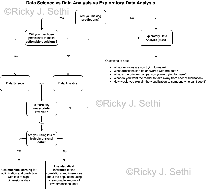
Nota Bene: these processes aren't disparate analyses and often form a pipeline from EDA → Data Analysis → Data Science, as discussed earlier; the above flowchart is only intended to determine when to use ML or Statistical Inference.
Sources of Error in Machine Learning
In supervised learning algorithms like decision trees, we can measure how well our machine learning model is performing by measuring the error in our model, which can also be thought of as how well it fits the problem and can be gauged using the signal to noise ratio. The signal of a dataset can be thought of as the underlying pattern we’re trying to discern while noise might be considered to be the randomness or irrelevant parts of the dataset. Generalization is the idea of how well a model can predict the signal on new data after being trained on known data.
Overfitting is when a model learns too much from the known, training data and is so customized to the known data that it performs poorly when faced with new, unseen data. An overfit model is usually too complex, with too many parameters or features, and starts capturing the noise and outliers in the training data. As such, an overfit model will perform well on training data but poorly on testing data. This often occurs with nonparametric and nonlinear models, like neural networks, SVMs, and decision trees, which usually contain parameters or techniques to limit how much detail the model learns.
Underfitting occurs when a model is too simple and doesn’t learn enough from the known, training data and so cannot generalize well on new data, either. An underfit model usually hasn’t seen enough data and might be too simple; in fact, it cannot even model the training data well and performs poorly in training. As such, it is easy to detect by using an appropriate performance metric and can be mitigated by increasing complexity or trying multiple machine learning algorithms. Simple models that cannot capture complex patterns in the data, like linear regression and logistic regression, often exhibit underfitting.
Although both underfitting and overfitting can be mitigated by trying multiple models, using cross-validation, or incorporating early stopping for algorithms with multiple iterations, overfitting is usually a more common problem in machine learning. We can help reduce the effects of overfitting by using regularization, which helps reduce the complexity of the model, and ensemble learning, which combines multiple algorithms. Underfitting and overfitting also exhibit a bias-variance tradeoff, where an increase in one results in a decrease in the other so a lot of supervised machine learning ends up tweaking the model to get a reasonable balance between underfitting and overfitting.
Variance error is how sensitive the model is to small fluctuations in the dataset. This is the error due to how much a target function's predicted value varies for a given training dataset. High variance is usually due to an overly-complex model that fits the training data too closely. Bias error measures how far off the predicted values are from the actual values and usually occurs when all the features are not taken into account. Bias error is thus the error that arises from incorrect assumptions in the algorithm, usually from a model with overly simplistic or faulty assumptions that cause it to miss important trends in the dataset’s features. Bias error can also be thought of as not being able to capture all of the signal in a dataset while variance error can be thought of as capturing too much of the noise in a dataset.
Models that overfit usually have high variance and low bias whereas underfitting models exhibit low variance and high bias. There is also an irreducible error, which is the noise that might be present regardless of which particular algorithm is used since it depends on things like missing variables, measurement imperfections, unknown forces, etc. Sometimes, data cleaning can help reduce this somewhat but usually there’s some effect from such noise that cannot be completely eliminated. The total error can thus be expressed as:
(Total Error) = (Bias Error)2 + (Variance Error) + (Irreducible Error)
Overfitting often occurs if your model does much better on the training dataset than the testing dataset. You can also check by using a very simple model as a benchmark to see if using more complex algorithms give you enough of a boost to justify their use. In general, to mitigate overfitting, you can:
Is Data Science a Science?
Before we tackle the idea of whether Data Science is a science or not, something that doesn’t seem to have a definitive answer, let’s step back and look at the idea of proof. This is a word that is overused quite frequently as there are many different kinds of proof: for example, there are scientific proofs, legal proofs, and mathematical proofs.
In mathematics, a proof is an inferential argument that shows a statement is true as supported by axioms, definitions, theorems, and postulates. Mathematicians normally use deductive reasoning to show that the premises, also called statements, in a proof are true. A direct proof is one that shows a given statement is always true and the proof is usually written in a symbolic language. In an indirect proof, mathematicians usually employ proof by contradiction, where they assume the opposite statement is true and eventually reach a contradiction showing the assumption is false.
In science, an inherently inductive enterprise,1 we cannot prove any hypothesis to be true as that would require an infinite number of observations so the best we can hope to do is use inductive reasoning as the basis of our generalization and hold it to be provisionally true. As noted by Lee Loevinger about Karl Popper, "In this view, which is fairly widely accepted, an hypothesis can be falsified, or disproved, but cannot be verified, or proved." Once it’s validated extensively and consistently, and we deem it to be sufficiently substantiated, we then call it a theory.
In law, legal proof is the process of establishing a fact by using evidence. In science, we might call this a validation of some theory as that usually also takes the form of an argument where you present a series of premises in support of some conclusion. Similarly to law, proof in science is usually limited to proof of facts in the sense of using data to establish the validity of facts. This is discussed at length by D.H. Kaye in [Kaye 1991] which shows that the use of quantitative observation-statements provide evidence to prove or, as we’d say in science, show the validity of, facts. So we could, in some sense, say that legal arguments use evidence to show the validity of a theory whereas science uses data to falsify a theory.
For example, following [Kaye 1991], collecting quantifiable data of the intensity and polarization of radiation at various frequencies from a radio telescope pointed at the Crab Nebula is the evidence that shows (in law, proves) something in the direction of the Crab Nebula is a radio source, the fact. Such facts can be deduced or induced from statements of observations, the evidence. Thus, a fact is based on some repeatable observation or measurement that is generally agreed upon to recur with the same value or in the same way under the same kinds of circumstances.
These facts are then used to inductively reason about a hypothesis or model of the system being studied. The predictions made by that model are further verified and, when enough predictions are verified independently, the hypothesis, or set of hypotheses, is considered sufficiently validated to be called a theory.
This process, this scientific method, is exactly what we employ when we utilize our machine learning models, like Hypothesis Testing in Section [sec:hypothesis-testing] or Decision Trees in Section [sec:learning-decision-tree], within a Data Science framework and use data to iteratively test and improve our models. I might further argue, following Feynman’s formulation, that as long as you’re using a systematic model to make predictions and then testing those predictions with data and using those results to validate or improve your model iteratively, you’re doing science.
Applying these scientific models to specific business problems2 without iteratively changing or further developing those models results in engineering and technology principles. As such, I might be inclined to categorize Data Analysis as an engineering discipline and Exploratory Data Analysis as a technological application.
Some Key Images
Some Key Images and corresponding Captions
Some key images and their corresponding captions from various chapters of the text.
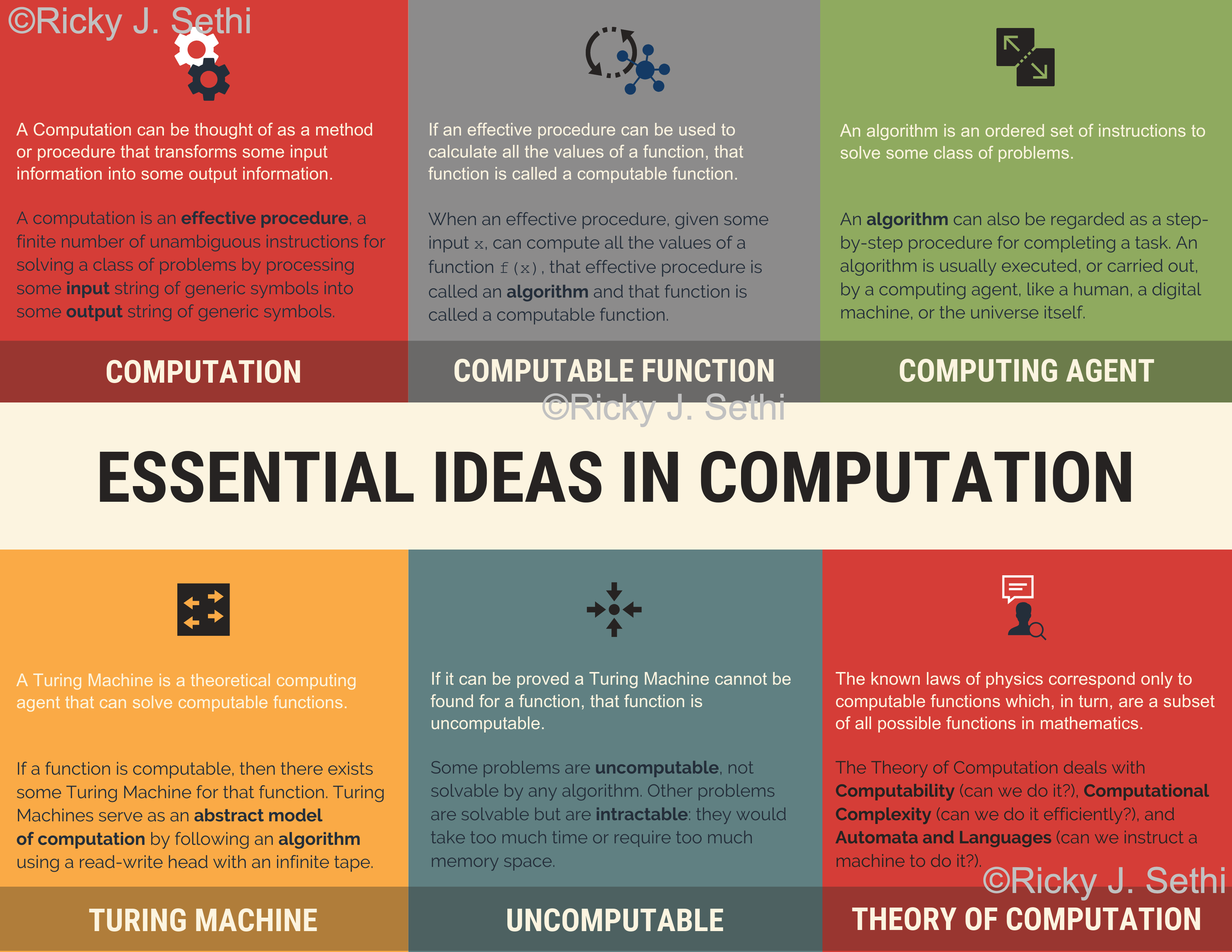
Caption: Some essential ideas in the theory of computation: an effective procedure is a finite set of instructions for carrying out some unambiguous symbolic manipulation or transformation. If an effective procedure can calculate all the values of a function, it is called an algorithm for that function and that function is then considered a computable function. A Turing Machine is a mathematical description of any algorithm in terms of a hypothetical machine with a simple read-write head and a tape of paper; a Turing Machine is one formalization of the general idea of an algorithm. In fact, computation itself can then be thought of as the study of algorithms or such formal models of algorithms.
Caption: Computational Thinking is a set of techniques for solving complex problems that can be classified into three steps: Problem Specification, Algorithmic Expression, and Solution Implementation & Evaluation. The principles involved in each step of the Computational Thinking Approach are:
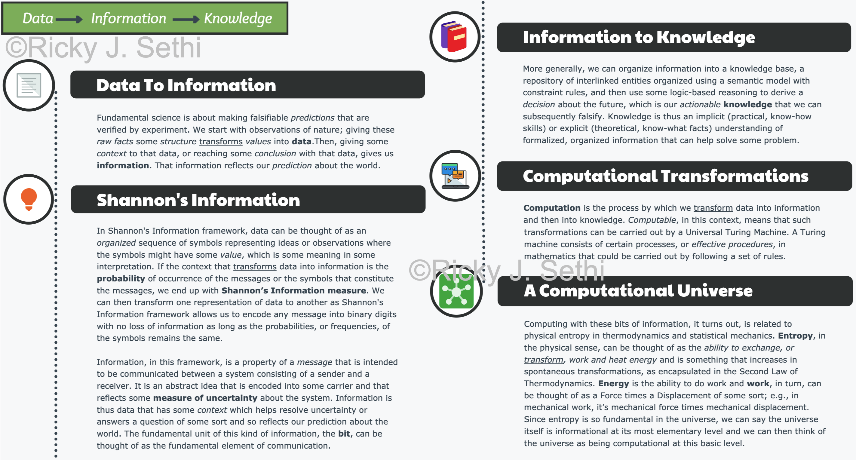
Caption: Data → Information → Knowledge
Fundamental science is about making falsifiable predictions that are verified by experiment. We start with observations of nature; giving these raw facts some structure transforms values into data.Then, giving some context to that data, or reaching some conclusion with that data, gives us information. That information reflects our prediction about the world.
In Shannon's Information framework, data can be thought of as an organized sequence of symbols representing ideas or observations where the symbols might have some value, which is some meaning in some interpretation. If the context that transforms data into information is the probability of occurrence of the messages or the symbols that constitute the messages, we end up with Shannon’s Information measure. We can then transform one representation of data to another as Shannon's Information framework allows us to encode any message into binary digits with no loss of information as long as the probabilities, or frequencies, of the symbols remains the same.
Information, in this framework, is a property of a message that is intended to be communicated between a system consisting of a sender and a receiver. It is an abstract idea that is encoded into some carrier and that reflects some measure of uncertainty about the system. Information is thus data that has some context which helps resolve uncertainty or answers a question of some sort and so reflects our prediction about the world. The fundamental unit of this kind of information, the bit, can be thought of as the fundamental element of communication.
More generally, we can organize information into a knowledge base, a repository of interlinked entities organized using a semantic model with constraint rules, and then use some logic-based reasoning to derive a decision about the future, which is our actionable knowledge that we can subsequently falsify. Knowledge is thus an implicit (practical, know-how skills) or explicit (theoretical, know-what facts) understanding of formalized, organized information that can help solve some problem.
Computation is the process by which we transform data into information and then into knowledge. Computable, in this context, means that such transformations can be carried out by a Universal Turing Machine. A Turing machine consists of certain processes, or effective procedures, in mathematics that could be carried out by following a set of rules.
Computation using these bits of information, it turns out, is related to physical entropy in thermodynamics and statistical mechanics. Entropy, in the physical sense, can be thought of as the ability to exchange, or transform, work and heat energy and is something that increases in spontaneous transformations, as encapsulated in the Second Law of Thermodynamics.
Energy is the ability to do work and work, in turn, can be thought of as a Force times a Displacement of some sort; e.g., in mechanical work, it’s mechanical force times mechanical displacement. Since entropy is so fundamental in the universe, we can say the universe itself is informational at its most elementary level and we can then think of the universe as being computational at this basic level.
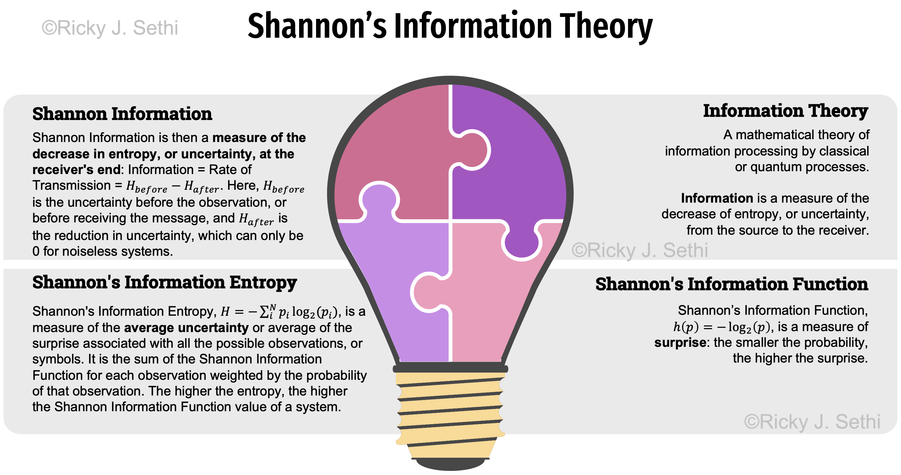
Caption: Shannon's Information Theory:
Information Theory is thus a mathematical framework that focuses on making choices, message transmission, and the state of systems. If the underlying processes are classical processes, the information processing framework is termed Classical Information Theory or Shannon's Information Theory. If those processes are quantum processes, then Quantum Information Theory deals with figuring out which information processing tasks are allowed by the quantum information carriers.
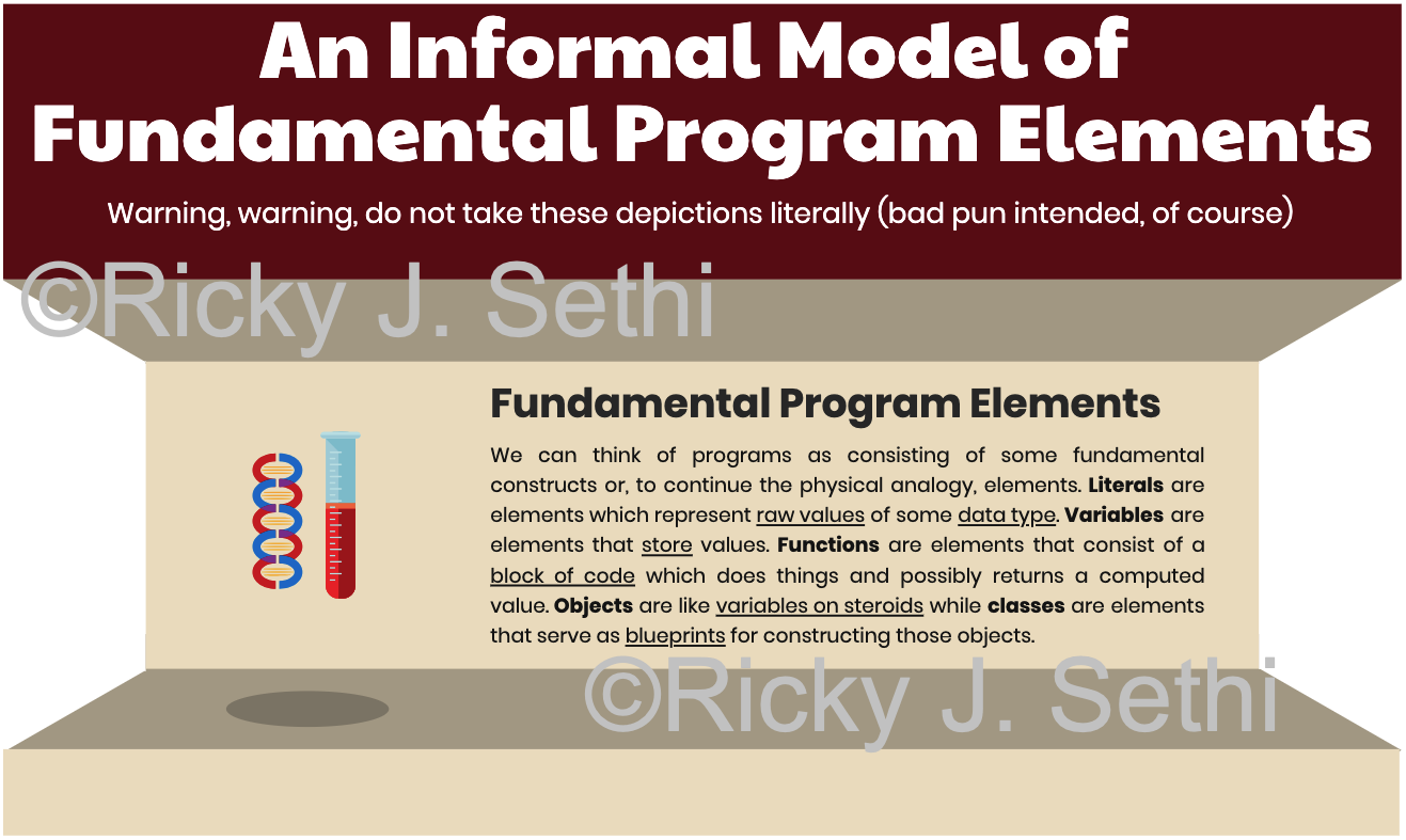
Caption: An Informal Model of Fundamental Program Elements: most programs consist of elements like literals, variables, functions, objects, and classes. Program statements are made up of expressions which contain elements. In addition, programs utilize control structures to determine the flow of execution, the order in which statements are executed. Three fundamental control structures, sequence, selection, and repetition, are sufficient to specify any programmatic solution. These control structures are implemented as statements; e.g., the selection control structure is implemented using the if statement in most programming languages.

Caption: Different Kinds of Errors: Syntax, Semantic, and Logical errors occur at either compile-time (syntax and static semantic) or run-time (dynamic semantic and logical). Semantic and logical errors are also sometimes referred to as exceptions and we can use exception handling to take care of such exceptional situations. Most languages use exceptions for both compile-time and run-time errors. In languages like Java, exceptions that occur at compile-time are called checked exceptions whereas run-time exceptions are called unchecked exceptions. In languages like Python, C++, and C#, the compiler does not force the programmer to deal with exceptions so all exceptions are unchecked.
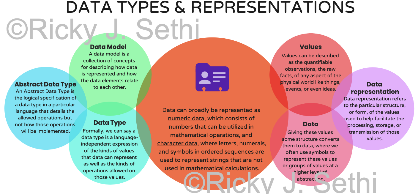
Caption:
Data Types and Representations:
Values can be described as the quantifiable observations, the raw facts, of any aspect of the physical world like things, events, or even ideas. Giving these values some structure converts them to data, where we often use symbols to represent these values or groups of values at a higher level of abstraction. Data representation refers to the particular structure, or form, of the values used to help facilitate the processing, storage, or transmission of those values.
Data can broadly be represented as numeric data, which consists of numbers that can be utilized in mathematical operations, and character data, where letters, numerals, and symbols in ordered sequences are used to represent strings that are not used in mathematical calculations. The kind of data, or its category as Aristotle might have said, is its type. Different types of data have different characteristics.
A data model is a collection of concepts for describing data that tells us how data is organized and represented. More formally, it is an abstract model that organizes how data is represented and how the data elements relate to each other. A type is the collection of values and a data type consists of the type along with the operations permitted to manipulate that type. A data type can also be thought of as a logical, language-independent expression of a data model and the associated operations that are valid on those data values, independent of any particular language.
The data type thus tells us both the kinds of values that data can represent as well as the kinds of operations allowed on those values. An abstract data type (ADT) is a data type that does not specify the details of how data will be organized in memory or which specific algorithms will be used for carrying out the operations on those data values. ADTs specify what operations can be performed on the data values but not how those operations will actually be implemented. While an ADT is the logical specification of a data type in some particular language but without the implementation details, a data structure is the actual implementation of that ADT in that particular language.
A variable is the name for a stored value that represents some fundamental characteristic of the system or function. More abstractly, a variable is any symbol used to represent an unspecified element chosen from some set of elements. These values and variables can be combined in expressions and those expressions combined further into statements, the instructions which make up an algorithm.
1Some might distinguish between an ADT Specification, which is more mathematical and language-independent, and is similar to a data type definition without any implementation details; an ADT Interface, which is language-dependent but still does not contain any implementation details and might be represented by a class or an abstract class in C++ or an interface class in Java; or a Concrete Data Type, which is language-dependent and includes the actual implementation of the ADT in that particular language.
Footnote: I should add the caveat that some might differ in the full extent of these meanings and often consider objects to be distinct from data structures. For example, you can implement an abstract data type as a data structure in a non-OO language like C using a pointer to a structure, struct. Some also endorse the perspective that an object only shows its functions (with data implied) while data structures only show the data (with the operations implied). However, what is hidden in an object, or its corresponding class, is usually a design decision by the programmer rather than a feature imposed by the language design. This is apparent in most languages like Java as they can have all their data elements publicly visible if they so choose and other classes can be data stores with no defined operations.

Caption:
Confusion Tables:
Confusion matrix with True Positive, True Negative, False Positive, and False Negative classifications. In a Hypothesis Testing framework, the null hypothesis, the statement we want to falsify, usually indicates there is no real effect. A false positive (α) is incorrectly rejecting the null hypothesis while a false negative (β) is incorrectly accepting the null hypothesis. Alpha, α, is the significance level used in Hypothesis Testing and Beta, β, is used to determine the statistical power of a study, which is the probability that it rejects a false negative, 1 - β.
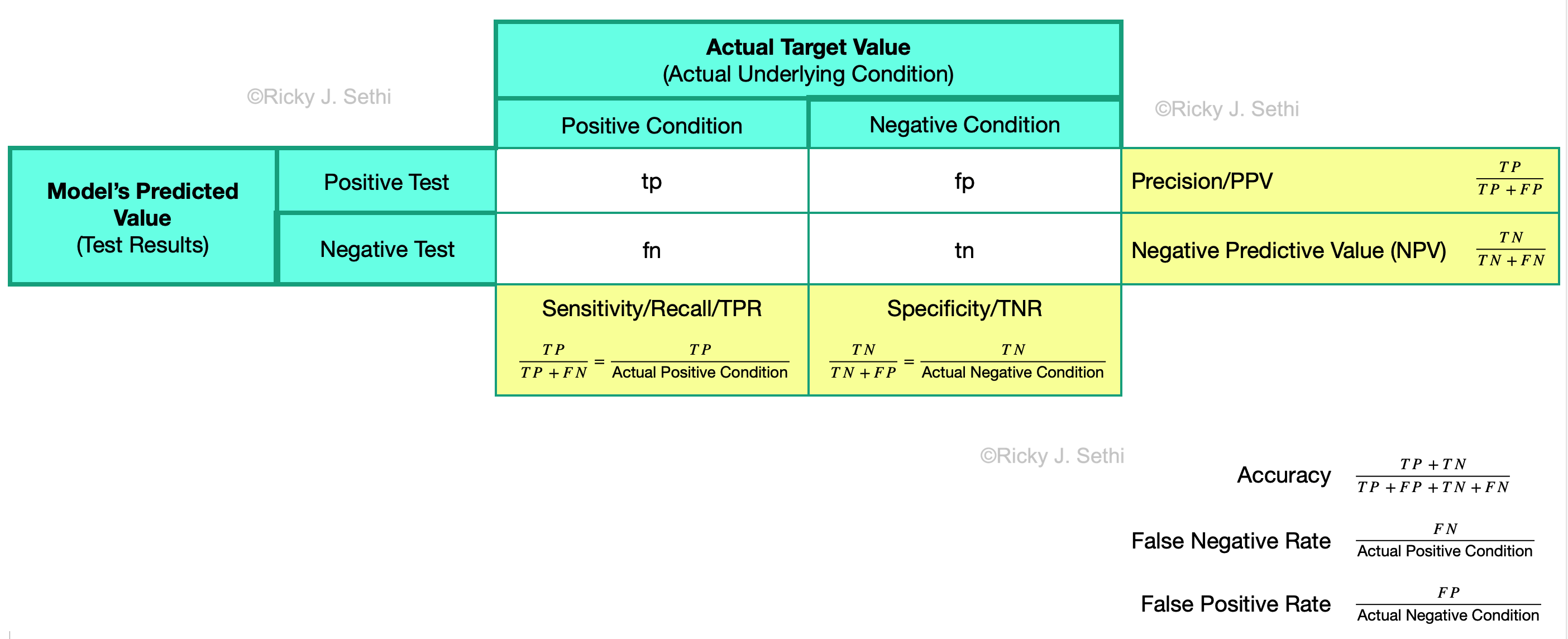
Caption:
Confusion Table Statistics:
Statistics computed using confusion tables, including Precision, Recall, Accuracy, Specificity, Sensitivity, etc. Here, tp is True Positive, tn is True Negative, fp is False Positive, and fn is False Negative. Finally, PPV is Positive Predictive Value, NPV is the Negative Predictive Value, TPR is the True Positive Rate, and FPR is the False Positive Rate. You can think of Recall as being the number of positive instances we actually retrieved and Precision as indicating how many of the instances we retrieved were actually positive.
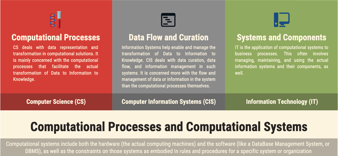
Caption:
Difference between CS, CIS, and IT:
Difference between Computer Science (CS), Computer Information Systems (CIS), and Information Technology (IT), three of the sub-fields of computation.
CS deals with data representation and transformation in computational solutions. It is mainly concerned with the computational processes that facilitate the actual transformation of Data to Information to Knowledge.
Information Systems help enable and manage the transformation of Data to Information to Knowledge. CIS deals with data curation, data flow, and information management in such systems. It is concerned more with the flow and management of data or information in the system than the computational processes themselves.
Computational systems include both the hardware (the actual computing machines) and the software (like a DataBase Management System, or DBMS), as well as the constraints on those systems as embodied in rules and procedures for a specific system or organization.
IT is the application of computational systems to business processes. This often involves managing, maintaining, and using the actual information systems and their components, as well.
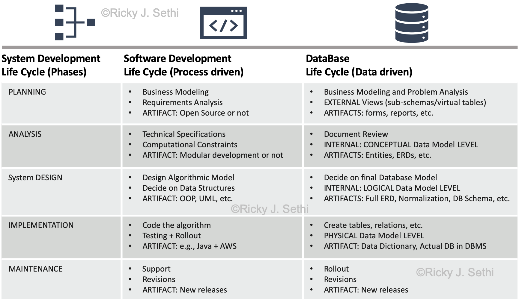
Caption:
DataBase Life Cycle:
Comparison of Systems Development Life Cycle, Software Development Life Cycle, and DataBase Life Cycle.
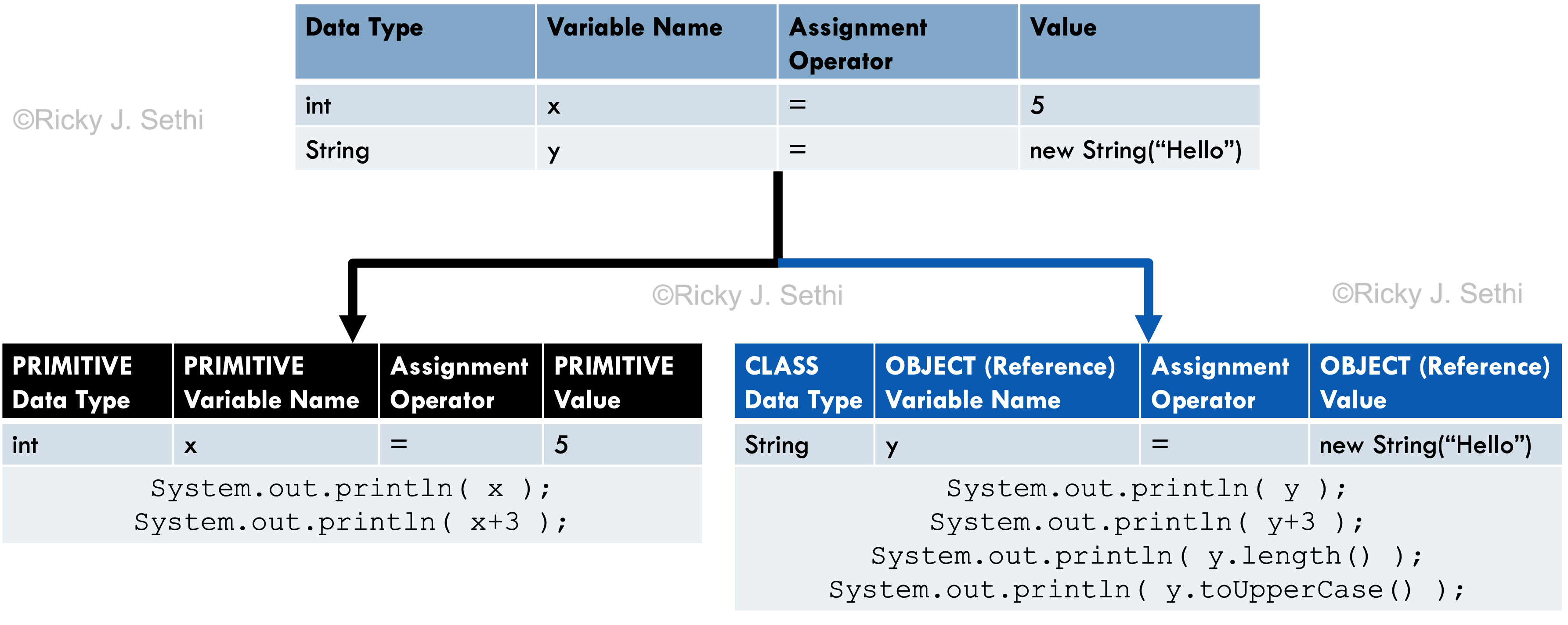
Caption:
Object Reference Variable vs Primitive Variable:
A Primitive Variable can only hold a value. An Object (Reference) Variable, though, is like a super-hero variable with powers and abilities far beyond those of Primitive Variables. When compared to a Primitive Variable, it can do things to the value it holds by invoking the methods defined in that Class Data Type.
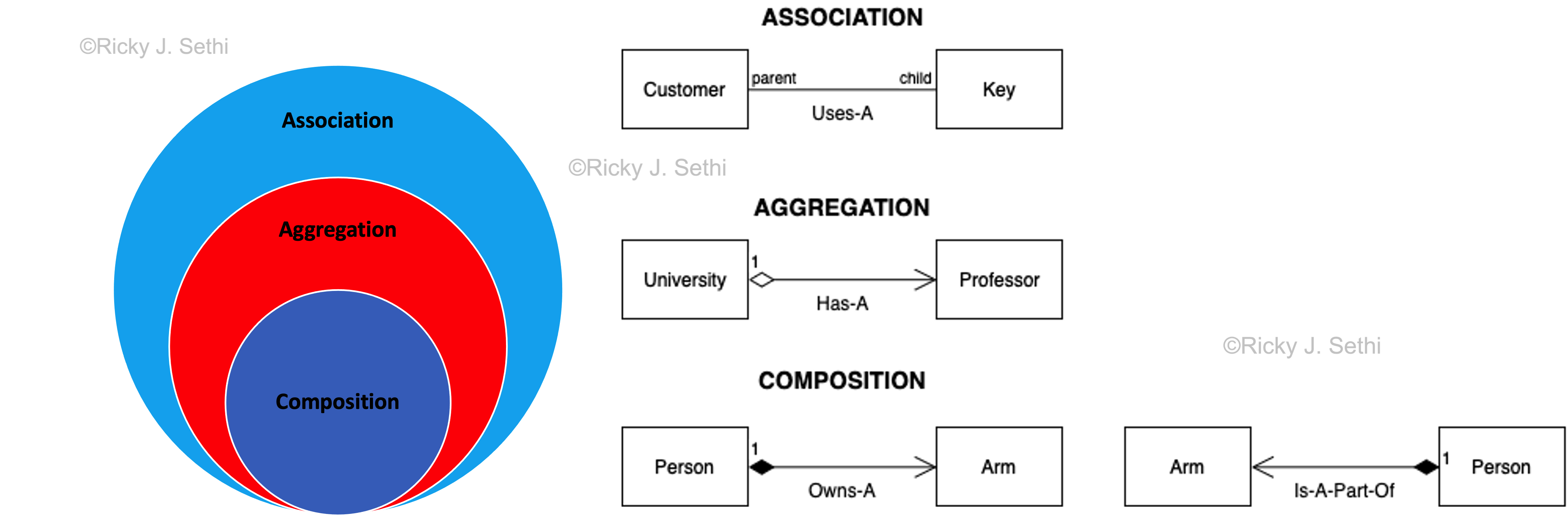
Caption:
Association, Aggregation, and Composition:
Association, Aggregation, and Composition and their associated UML diagram representations.
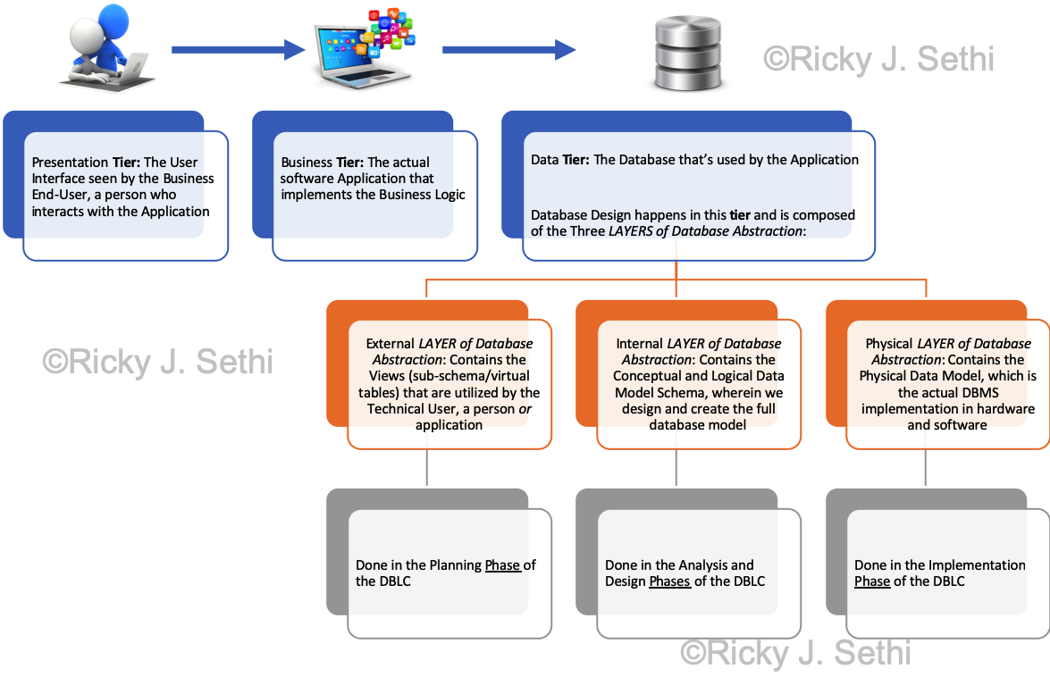
Caption:
Tiers, Layers, and Phases:
Three-Tiered Client-Server Application Architecture, Layers of Database Abstraction, and DataBase Life Cycle Phases.
This is the Three-tiered client-server database Application Architecture. It shows the Application Development Tiers and their relationship to the Layers of Database Abstraction, as well as the DataBase Life Cycle (DBLC) Phases.
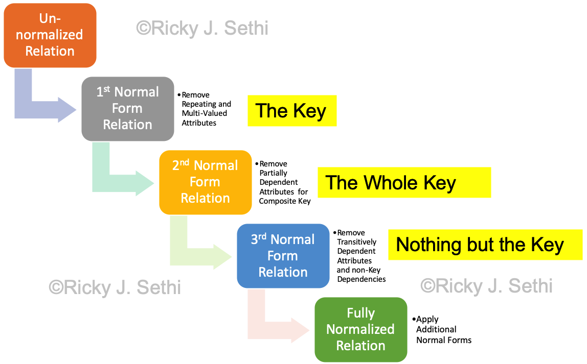
Caption:
Database Normalization:
Database Normalization Overview: "The Key, the whole Key, and nothing but the Key".
Database Normalization: At each step, we create more tables/entities. We also see the guiding maxim of database normalization, "The key, the whole key, and nothing but the key," for getting to the 3rd Normal Form (NF).
1NF: No repeating attributes or multi-value attributes.
2NF: No partial dependencies with a composite key or no composite key at all.
3NF: No transitive dependencies on non-key attributes.
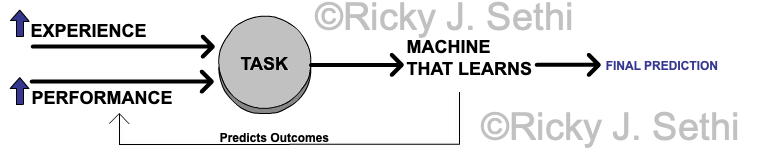
Caption:
Machine Learning Definition:
Following Alan Turing and Tom Mitchell's ideas, one definition of Machine Learning can be: a Machine, or a computer program, is said to Learn if its Performance at a Task improves with Experience. The Experience is the input Data and the Performance is quantified by a Performance Measure. Once its performance is sufficient, it outputs a final prediction, the result of its learning.
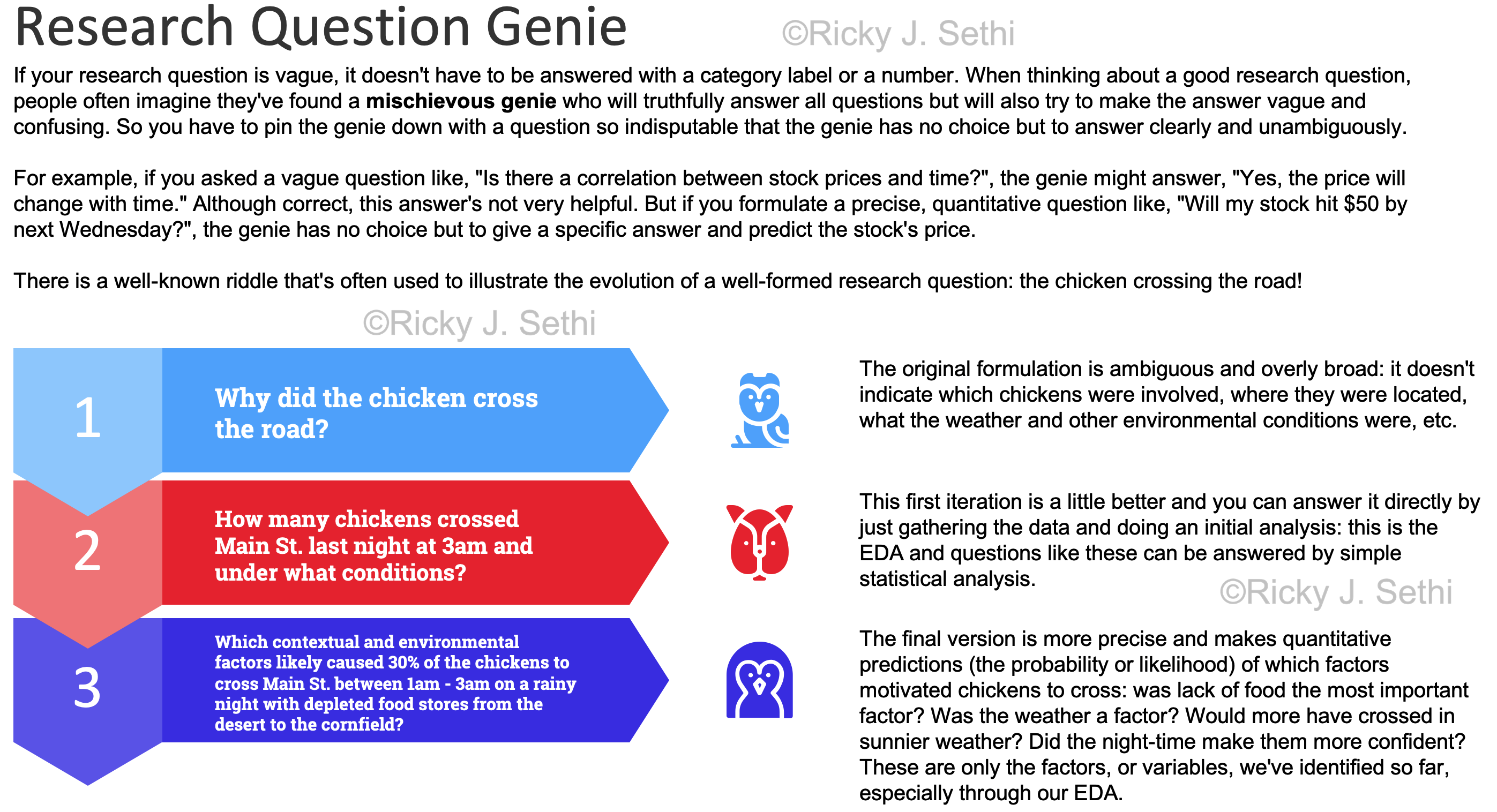
Caption:
Research Question Genie:
If your research question is vague, it doesn't have to be answered with a category label or a number. When thinking about a good research question, people often imagine they've found a mischievous genie who will truthfully answer all questions but will also try to make the answer vague and confusing. So you have to pin the genie down with a question so indisputable that the genie has no choice but to answer clearly and unambiguously.
For example, if you asked a vague question like, "Is there a correlation between stock prices and time?", the genie might answer, "Yes, the price will change with time." Although correct, this answer is not very helpful. If, on the other hand, you formulate a precise, quantitative question like, "Will my IBM stock hit $50 by next Wednesday?", the genie has no choice but to give a specific answer and predict the stock's price.
There is a well-known riddle that's often used to illustrate the evolution of a well-formed research question: the chicken crossing the road!
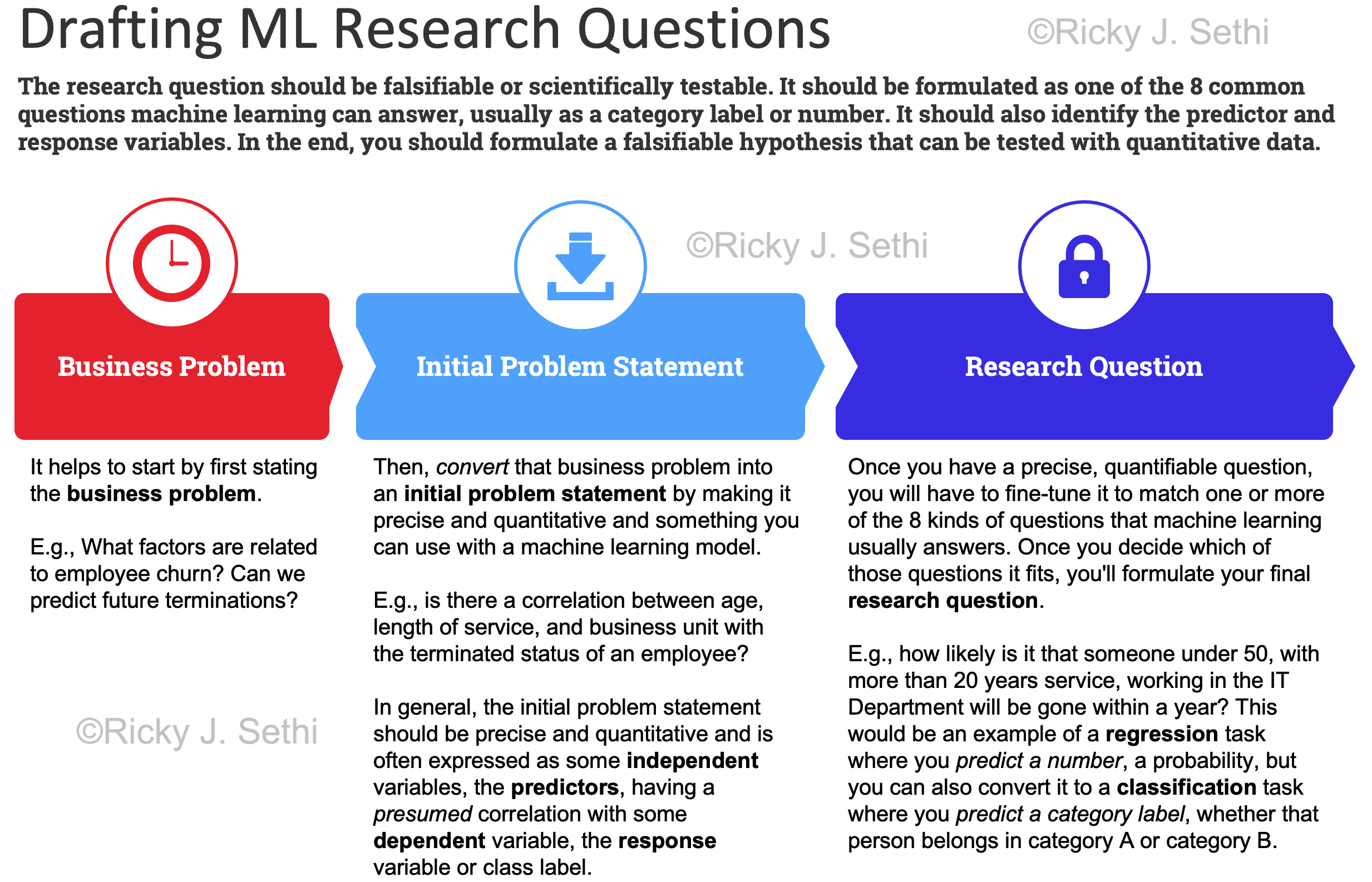
Caption:
Drafting Machine Learning Research Questions:
The research question should be falsifiable or scientifically testable. It should be formulated as one of the 8 common questions machine learning can answer, usually as a category label or number. It should also identify the predictor and response variables. In the end, you should formulate a falsifiable hypothesis that can be tested with quantitative data.
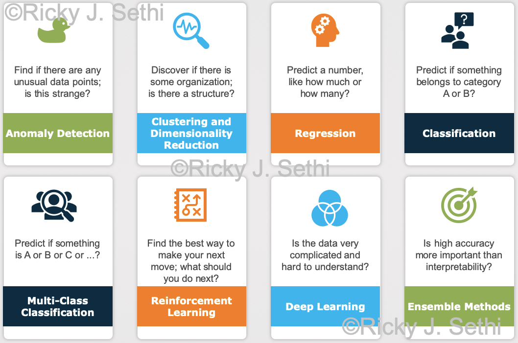
Caption:
Eight Common ML Approaches:
Pragmatically speaking, there are usually eight kinds of questions
we answer in most data analytic applications. Each of these eight
questions is usually addressed using a different machine learning
algorithm. These eight common questions and their corresponding
approaches are:
We usually start by stating the business problem. E.g., What factors are related to employee churn? Can we predict future terminations? We then convert that business problem into a research problem statement by making it precise and quantitative and something you can use with a machine learning model. E.g., is there a correlation between age, length of service, and business unit with the terminated status of an employee?
In general, the research problem statement should be precise and quantitative and is often expressed as some independent variable(s) (the predictor(s)) having a presumed correlation with some dependent variable (the response variable or class label). Once we have a precise, quantifiable research question, we can see if it matches one or more of these questions that machine learning usually answers.
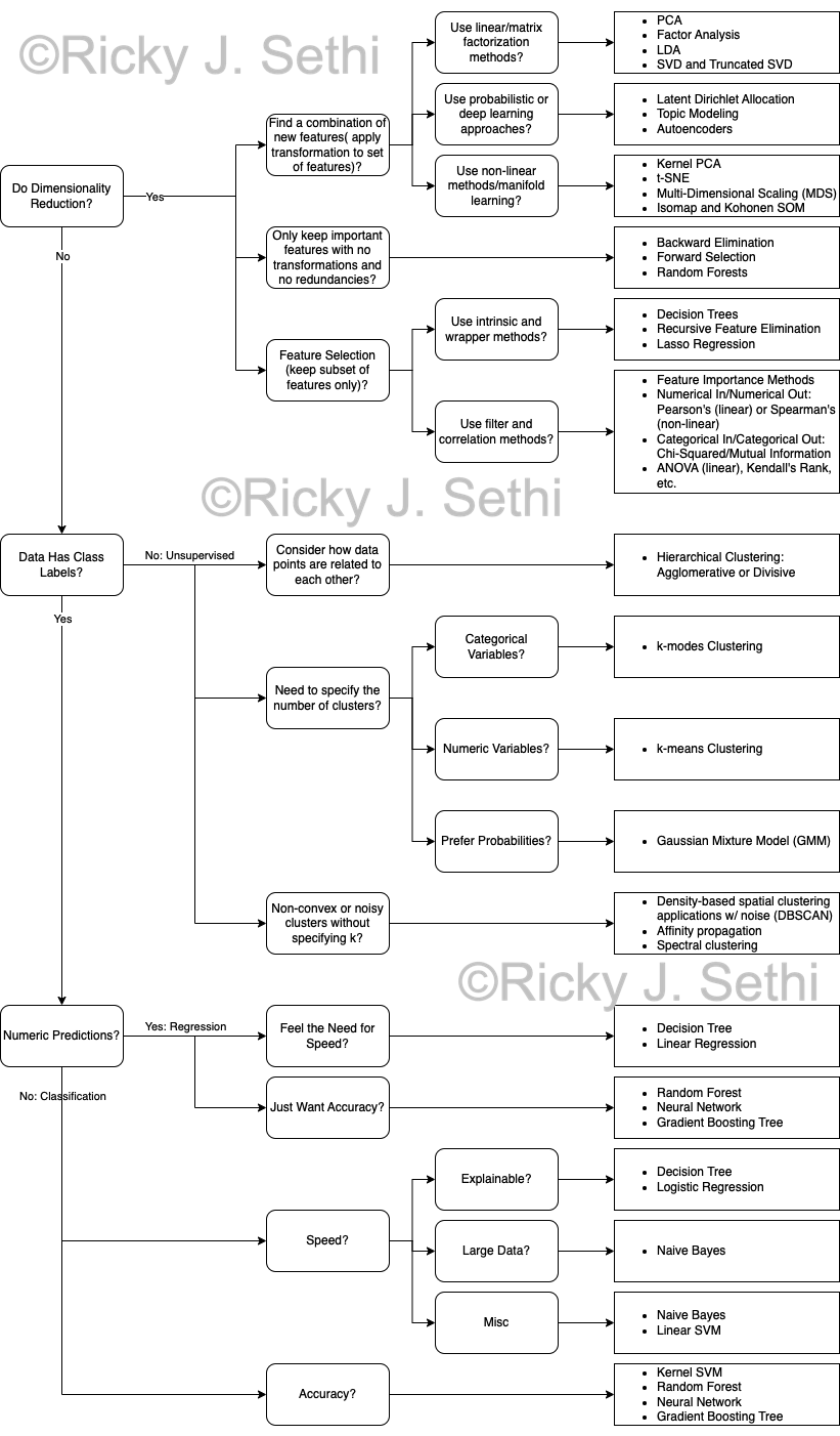
Caption: Selecting a Machine Learning Algorithm flowchart:
A general overview of how to pick a machine learning algorithm.
A good general approach to doing machine learning is to:
These are just some heuristics, or potential approaches, which is highly dependent on the kind of dataset as well as the size and quality of the data itself as well as any underlying distributions for any of the features. Equally important as selecting the right machine learning algorithms is picking the right metrics for them, and whether the accuracy or interpretability or ease of implementation/deployment is most important.
In addition to our unsupervised and supervised learning approaches above, there are also semi-supervised and reinforcement learning approaches that aren't covered in that flowchart.
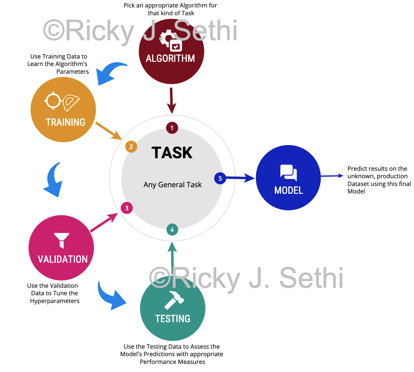
Caption: General Supervised Learning approach: Supervised learning approach for a general predictive model:
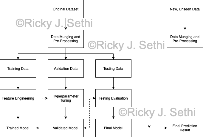
Caption: Supervised Learning Dataflow Overview for a general predictive model:
The overall process is something akin to:
Caption: Data Science Flowchart: We can analyze data in three fundamental ways:
Depending on the answers, you can eventually use either machine learning for optimization and prediction with lots of high-dimensional data or statistical inference to find correlations and inferences about the population using a reasonable amount of low-dimensional data.
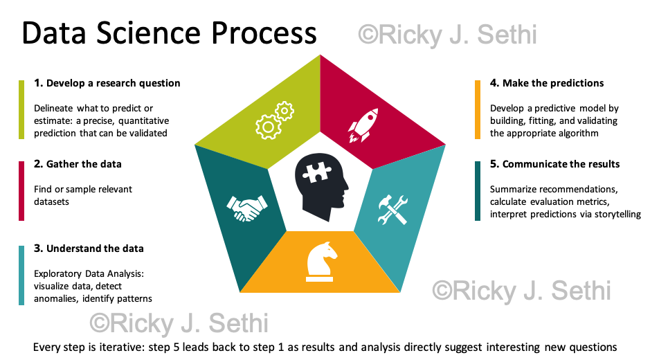
Caption: Data Science Process:
Every step of this process is iterative so, as Tom Jones is wont to say, it's not unusual to revisit any previous step; in fact, step 5 inevitably leads back to step 1 as your results and analysis usually lead directly to interesting new questions to ask.
In order to come up with the research question, you'll often start with EDA and summarization; e.g., you might summarize the average GPA of students. Then, look for relations or covariances or inferences: is amount of sleep related to change in GPA? Finally, make a prediction: does more than 8 hours of sleep increase GPA by 0.3 points over the average GPA?
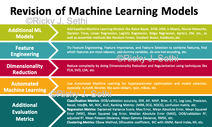
Caption: Revising ML Models:
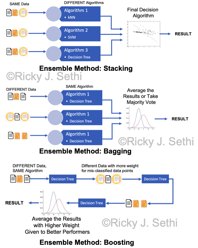
Caption: Ensemble methods: Stacking, Bagging, and Boosting:
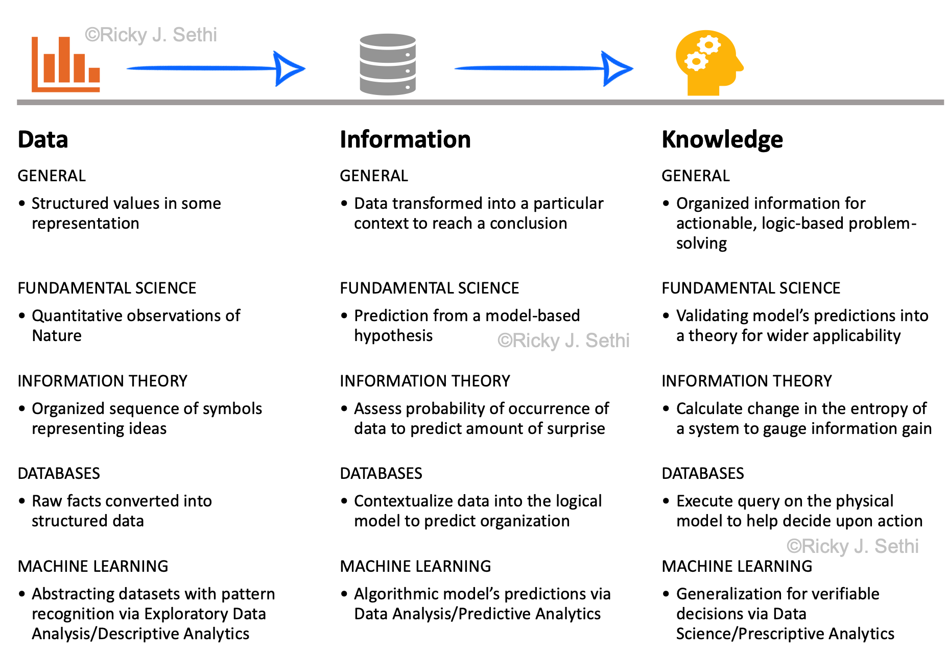
Caption: To summarize, then:
Final Data → Information → Knowledge Paradigm for five cases:
| Data → | Information → | Knowledge |
|
|
|
|
Errata
In Order, by Page and Figure Numbers
Profile

Curriculum Vitae (CV)
Profile Summary
- Affiliations:
- Fitchburg State University
- Worcester Polytechnic Institute
- Southern New Hampshire University
- Education:
- University of California, Berkeley
- University of Southern California
- University of California, Riverside
- Field of Research:
- Social Computing
Fact-checking misinformation, virtual communities, and group collaboration for science learning - Data Science
Multimedia analysis in digital humanities, deep learning for IR and XAI, and reproducibility via semantic workflows - Computer Vision
Group analysis in video using physics-based, machine learning models
- Social Computing